4.2 Orthomosaic creation and data preparation for analysis

The generation of a multispectral orthomosaic and its subsequent analysis constitute the next stage in the processing workflow, following image import and preliminary data preparation. This stage provides the basis for calculating spectral indices and assessing crop conditions.

Once all multispectral images have been imported and the processing parameters configured, the orthomosaic can be generated by processing and combining the overlapping images. The orthomosaic is a key output of photogrammetric processing and serves as the basis for subsequent agricultural land analysis. It represents a continuous, georeferenced image of the surveyed area created by combining multiple overlapping aerial photographs. Unlike individual aerial photographs, an orthomosaic is geometrically corrected to minimise perspective-related distortions and provide spatially consistent measurements. Its georeferenced pixels can be used to measure distances and areas, assess vegetation conditions, and calculate spectral indices.

To initiate processing, the user clicks “Start Processing” (Figure 52). From this point, Pix4Dfields automatically initiates the photogrammetric data processing; no further action is required from the user, as the software performs all calculations autonomously. During processing, a progress bar and the current operational stage are displayed at the bottom of the window (Figure 53). In this phase, the software determines the position of the photographs, matches common features, eliminates geometric distortions, and generates a continuous image of the terrain while maintaining the spatial alignment of all spectral bands.

Once processing is complete, the resulting orthomosaic is displayed (Figure 54), which offers several significant advantages over individual photographs: the entire territory is represented in a single image, perspective distortions are absent, every pixel has geographical coordinates, and the original spatial resolution of the survey is preserved. Consequently, the resulting data can be used for further analysis. The orthomosaic contains discrete spectral bands: blue, green, red, red edge, and near-infrared, which are used in the generation of vegetation index maps.

The project layers are displayed in the left-hand panel. In the workflow described here, a surface model is also available alongside the orthomosaic. Selecting the orthomosaic opens its corresponding tools in the right-hand panel. The “View” section displays the layer type, the colour channel scheme, the colours used, and their descriptions (Figures 55, 56).

The “Annotations” section provides tools for displaying markers, labels, and sketches (Figure 57), as well as importing geometric data (Figure 58). The “Info” section provides information about the layer, including its area, dimensions, ground sampling distance (GSD), file size, data type, creation time, processing workflow, value ranges, survey time, and coordinate reference system (Figure 59).

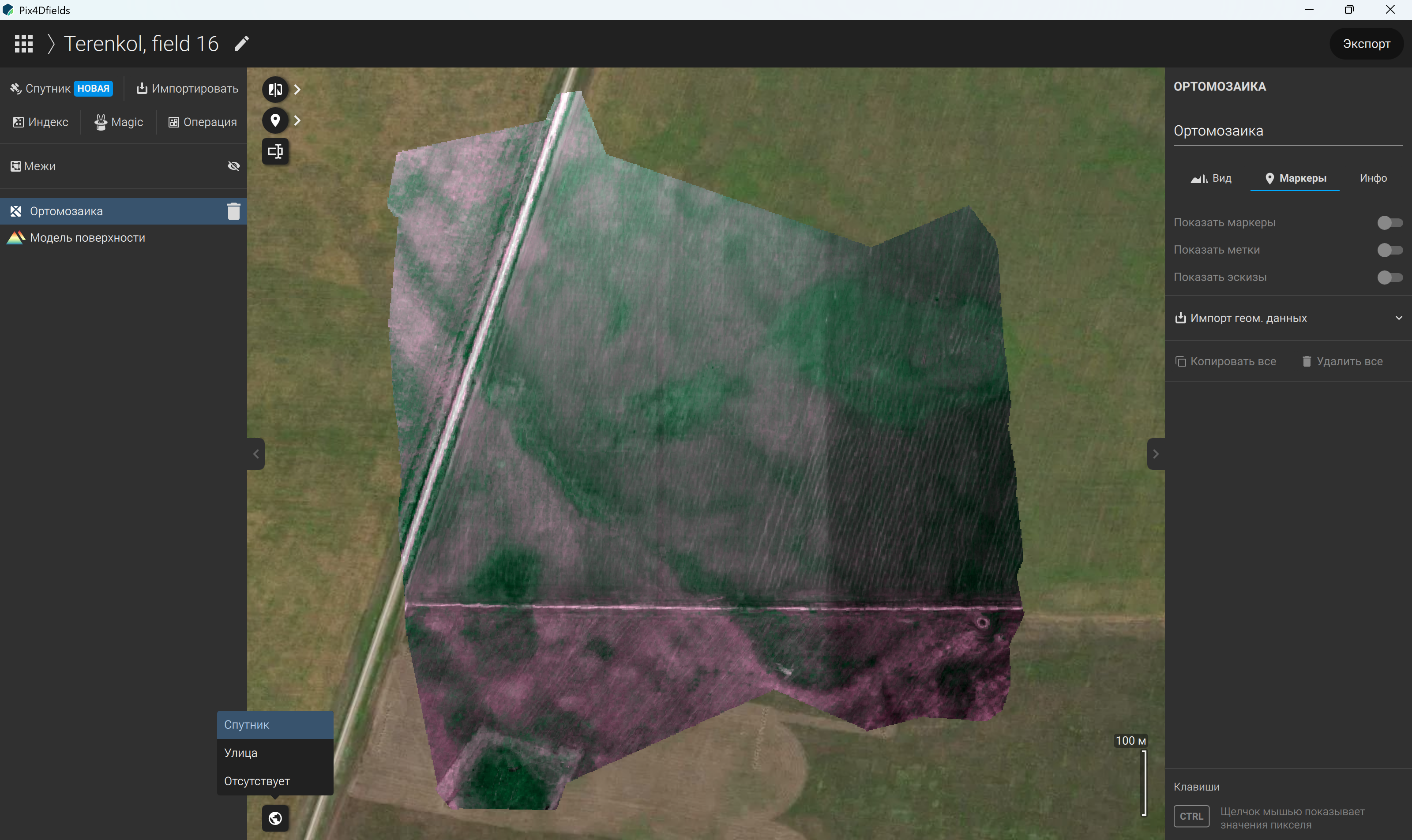
Figure 54 – Generating an orthomosaic from stitched images and selecting a basemap

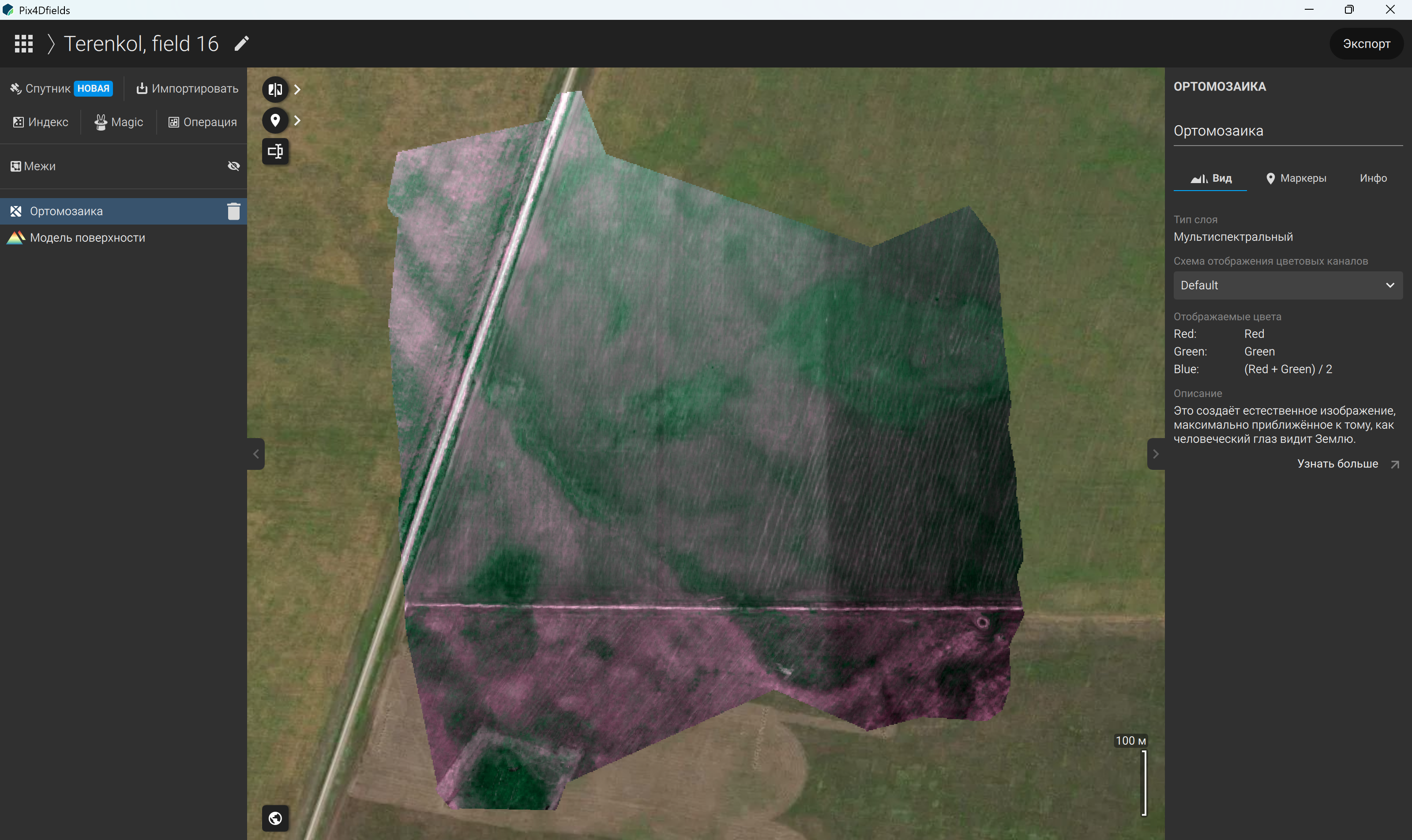
Figure 55 – “View” section of the orthomosaic layer in the right-hand panel

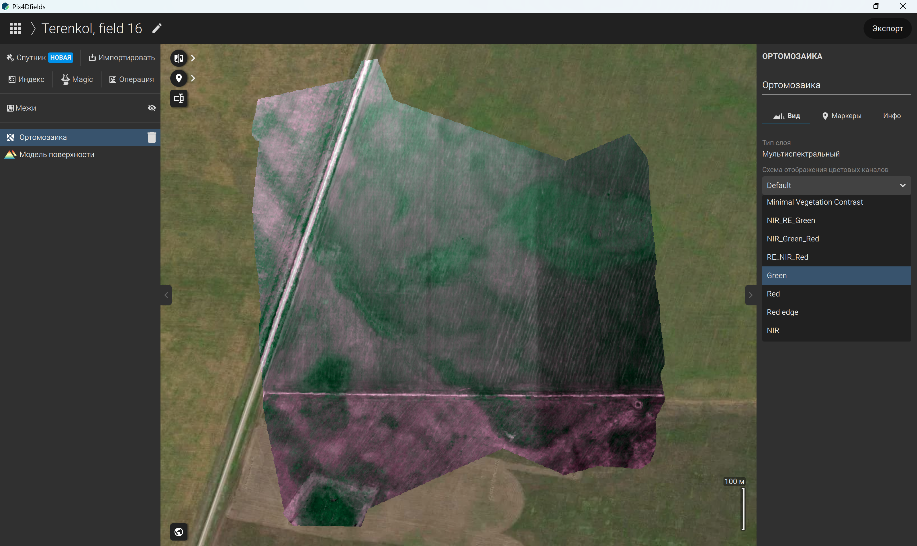
Figure 56 – Colour channel display settings in the “View” section of the right sidebar for the orthomosaic layer

When the surface model is selected, the contents of the right-hand panel change accordingly. In the “View” section (Figure 60), an elevation histogram is displayed below the visualisation options. A slider beneath the histogram allows the user to adjust the elevation range represented in the display, with the left and right limits corresponding to the lower and upper elevation thresholds, respectively (Figure 61). A corresponding histogram is also displayed at the bottom of the map view. The “View” section provides several colour schemes for visualising the surface model, including Greyscale (Figure 62), Red-Green (Figure 63), Glow (Figure 64), and Turbo (Figure 65). The intensity of the colour overlay can also be adjusted. The “Histogram Equalisation” option enhances the visual distinction between elevation values, making relatively small variations easier to identify (Figure 66). Manual adjustment of the histogram parameters is also available (Figure 67), allowing the user to customise the elevation range and its visual representation. In the selected colour configuration, higher elevations are represented by red and orange tones, whereas lower elevations are indicated by blue and purple tones. The elevation histogram can be used to examine the distribution of elevation values across the surveyed area and identify the relative prevalence of different elevation ranges. The surface model also includes an “Annotations” section (Figure 68), which allows geometric data to be imported (Figure 69). The “Info” section provides detailed information about the selected layer (Figure 70).

The “Boundaries” tool is located in the left-hand panel above the layer list (Figure 71). It enables field boundaries to be delineated manually or, where supported, automatically using artificial intelligence (AI). The tool also provides options for identifying and delineating obstacles within the surveyed area (Figure 72). The formation of field boundaries and the delineation of the border begin with defining the starting point (Figure 73), drawing the boundaries of one side (Figure 74), selecting the area (Figure 75), and conclude with the generation of the actual field boundaries (Figure 76). The resulting boundary can be measured (Figure 77) and edited if necessary (Figure 78). Once the boundary has been defined, it can be generated from the selected area and saved (Figures 79, 80, 81). The resulting boundary can then be used to define the area of interest within the orthomosaic (Figures 82, 83). Where supported, the same spatial selection can be applied to multiple layers simultaneously (Figure 84). This produces a boundary corresponding to the selected field area (Figure 85), allowing the map display to focus on the area of interest while excluding areas outside the selected boundary from the resulting field-specific view (Figures 86, 87).

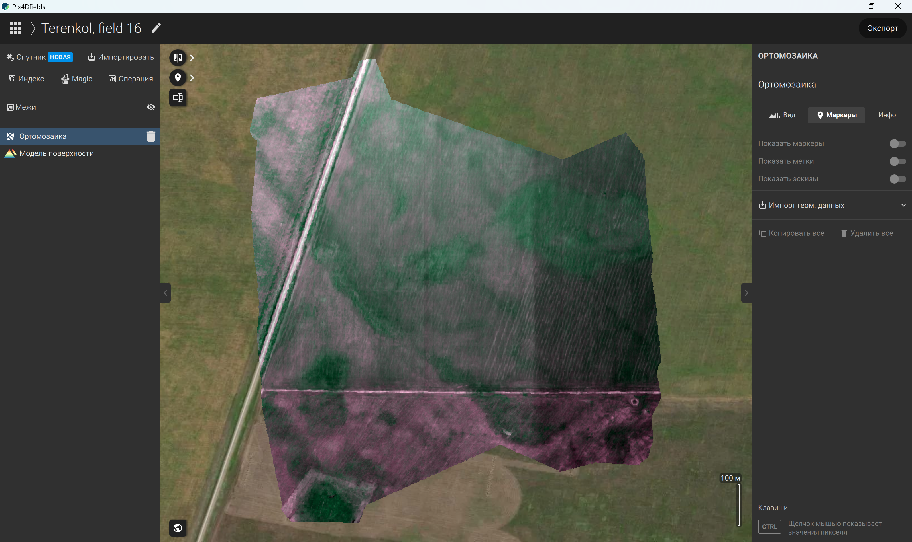
Figure 57 – “Annotations” section of the orthomosaic layer in the right-hand panel

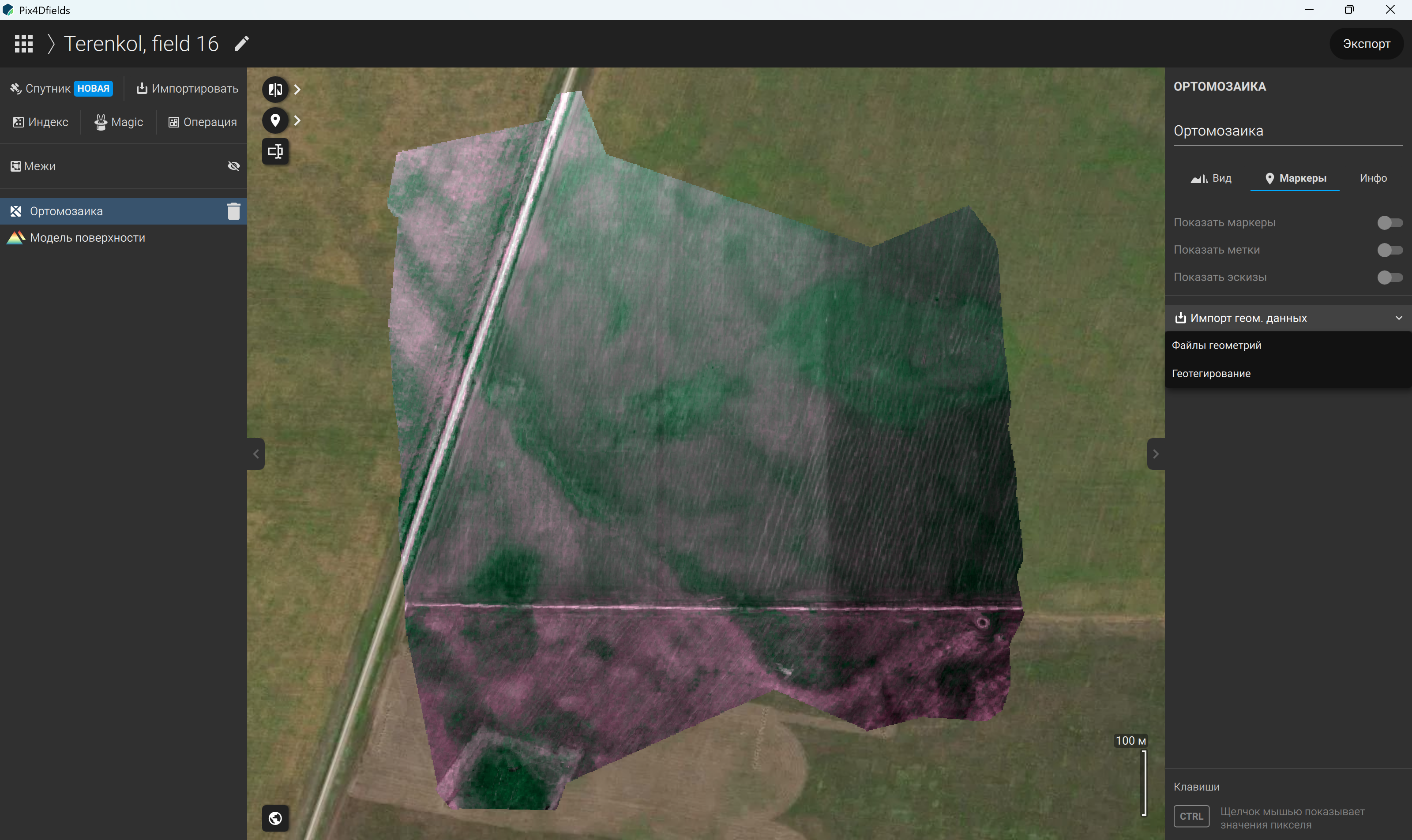
Figure 58 – Importing geometric data through the “Annotations” section of the orthomosaic layer

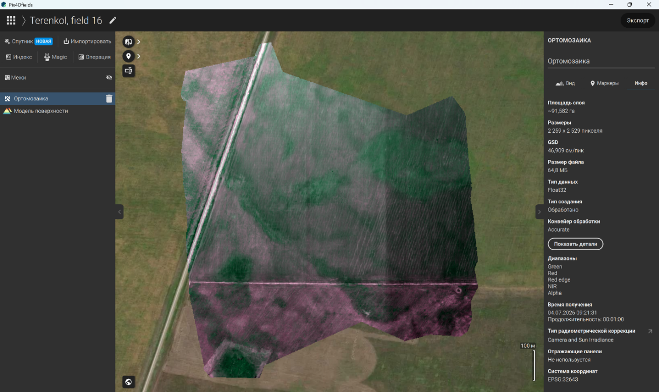
Figure 59 – “Information” displayed in the Info section of the orthomosaic layer

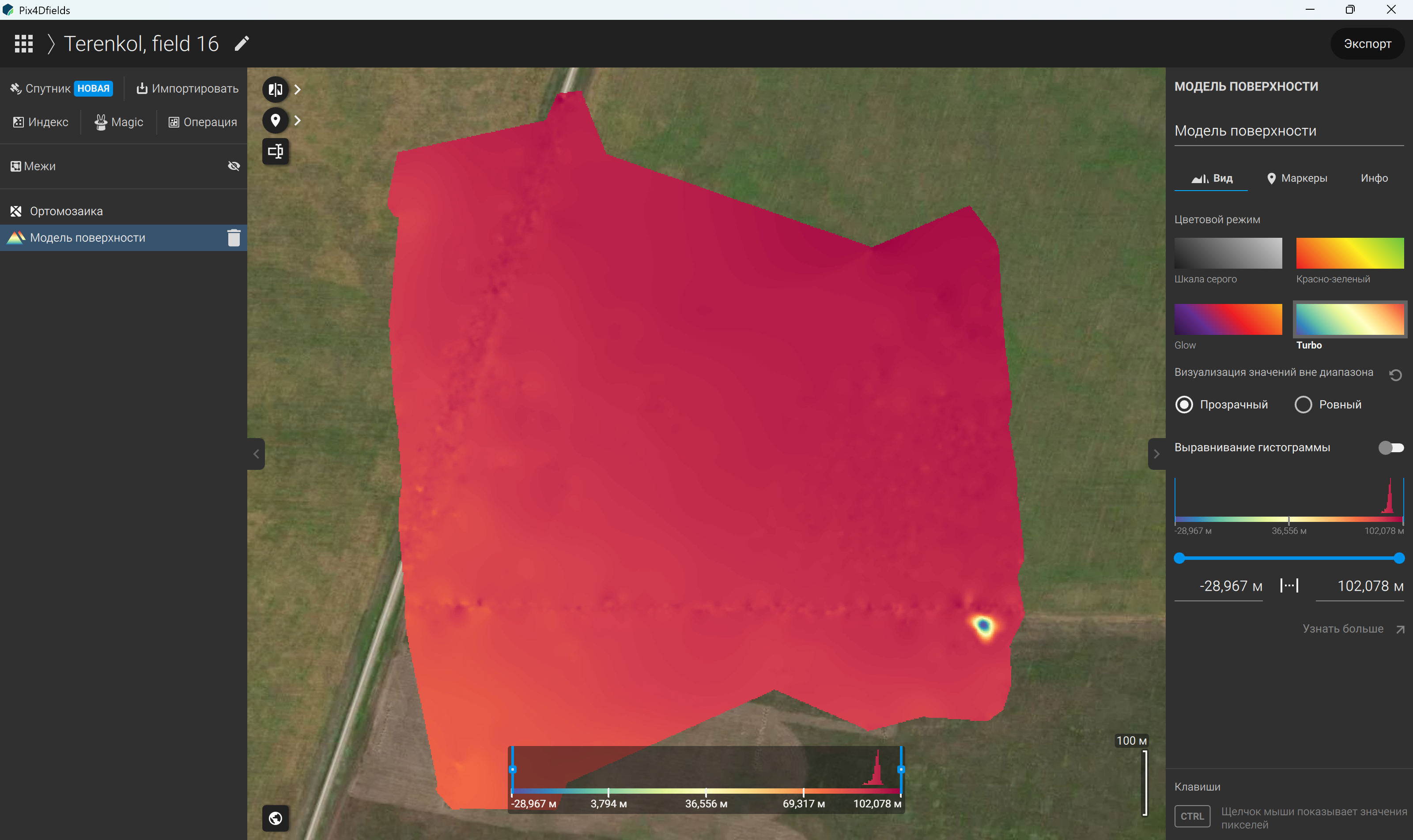
Figure 60 – “View” section of the surface model layer in the right-hand panel

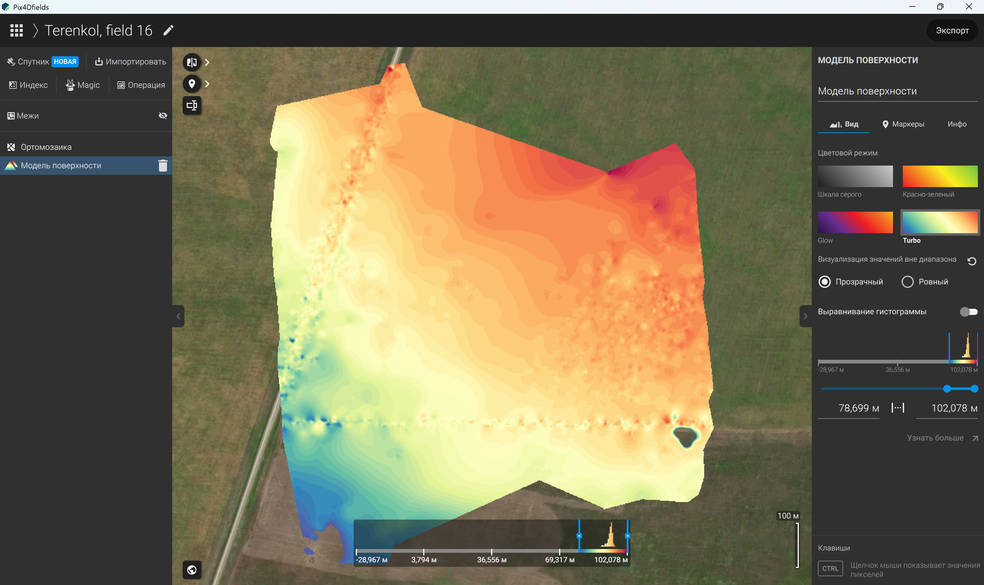
Figure 61 – Adjusting the elevation range using the histogram in the “View” section of the surface model layer

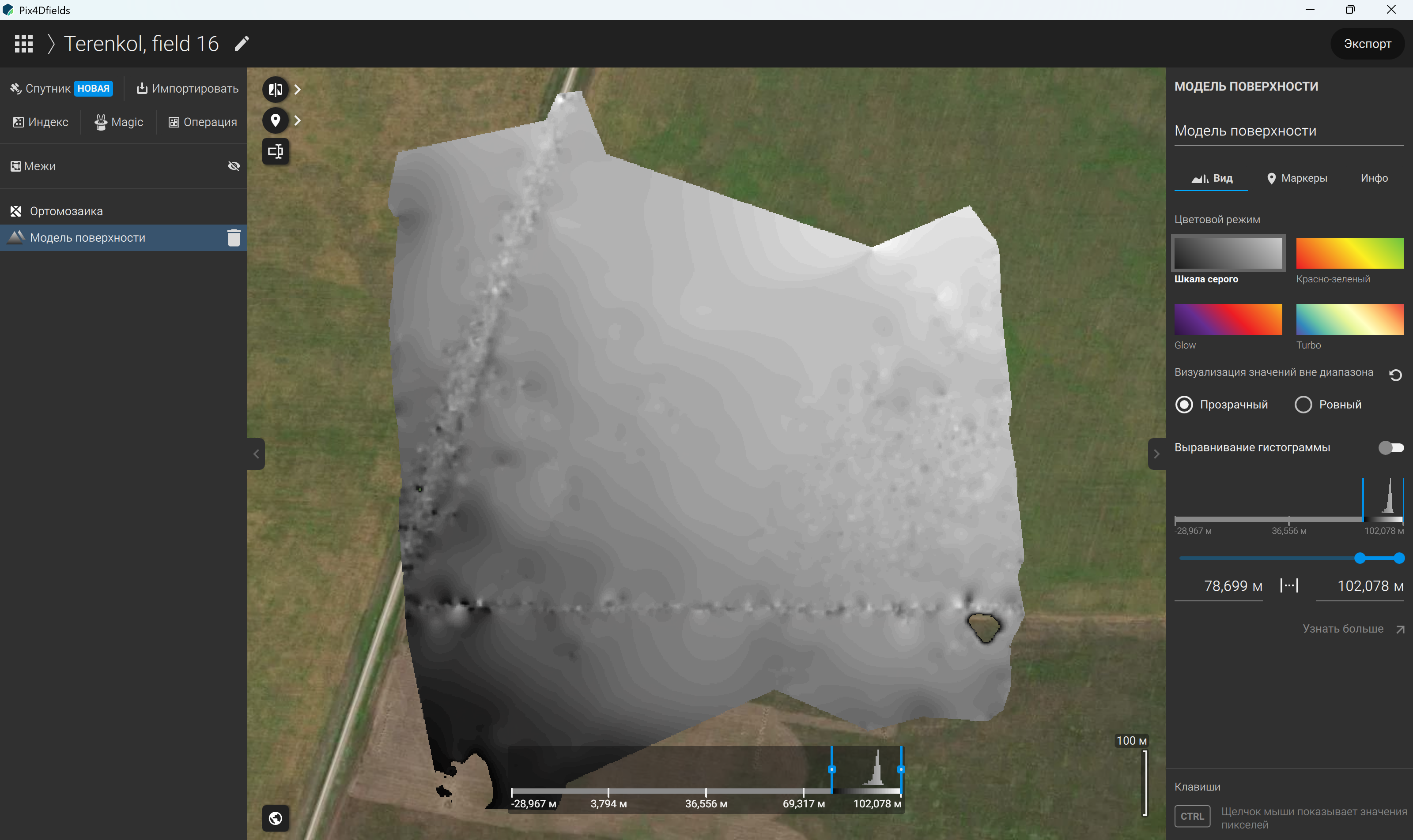
Figure 62 – Surface model visualised using the Greyscale colour scheme

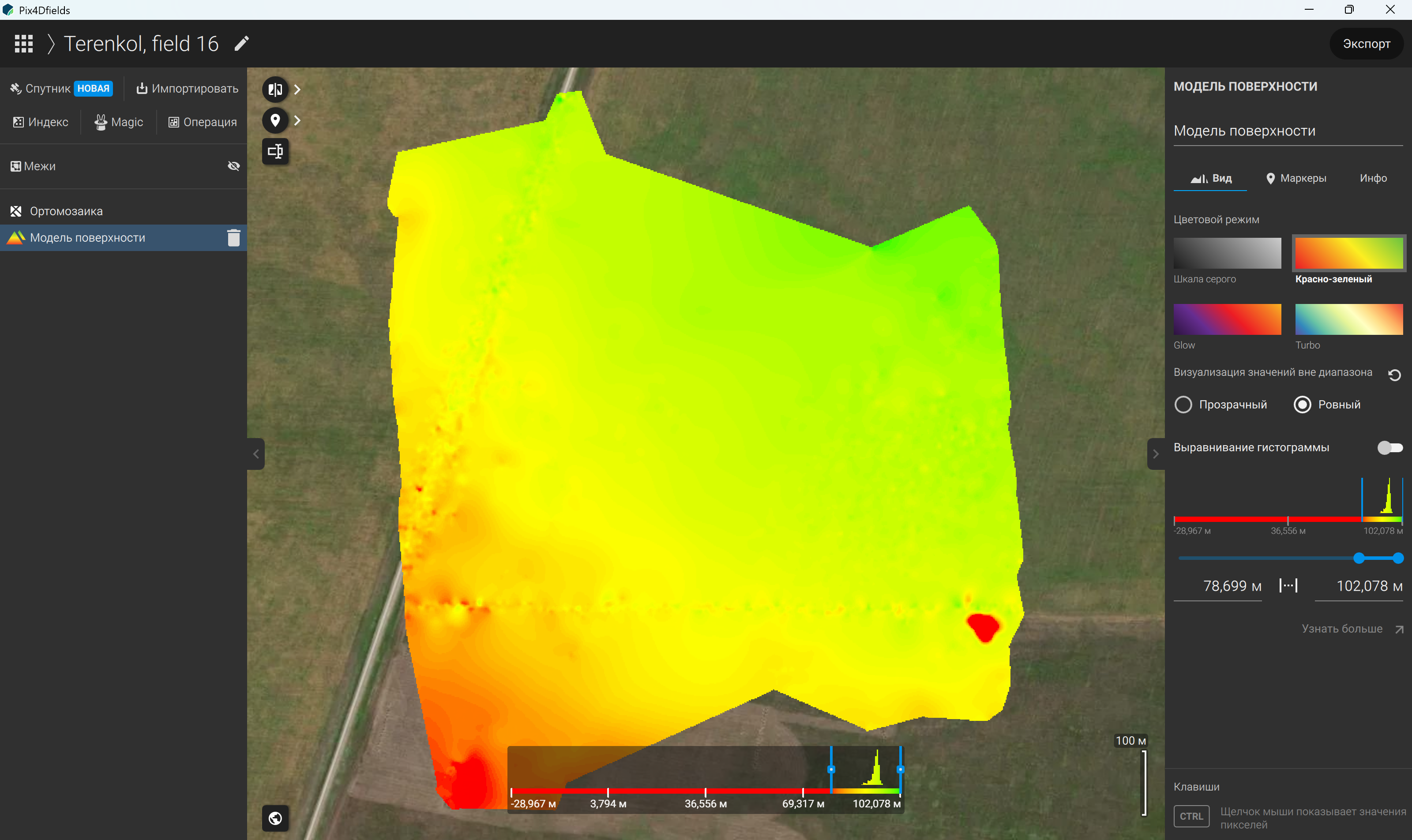
Figure 63 – Surface model visualised using the Red-Green colour scheme

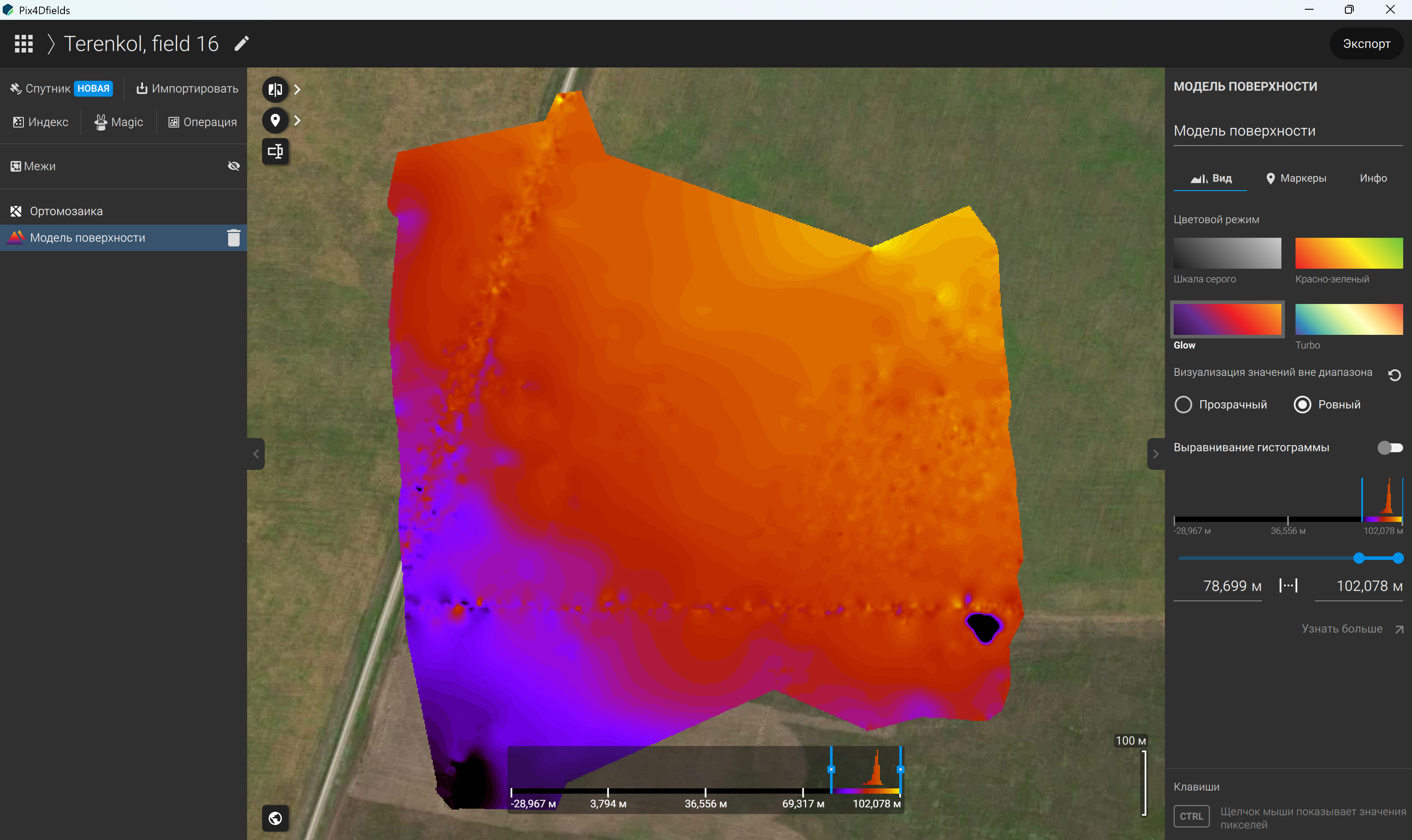
Figure 64 – Surface model visualised using the Glow colour scheme

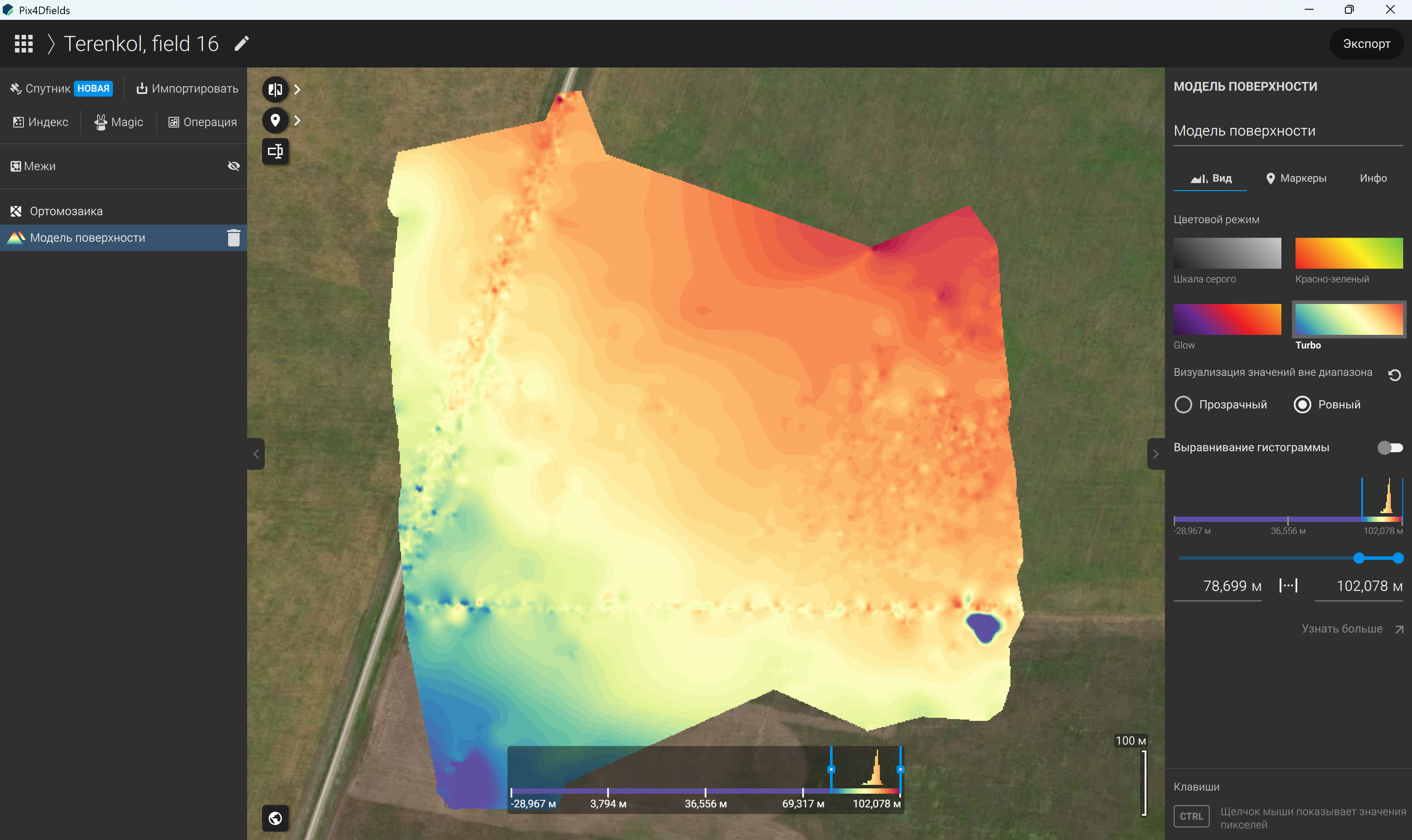
Figure 65 – Surface model visualised using the Turbo colour scheme

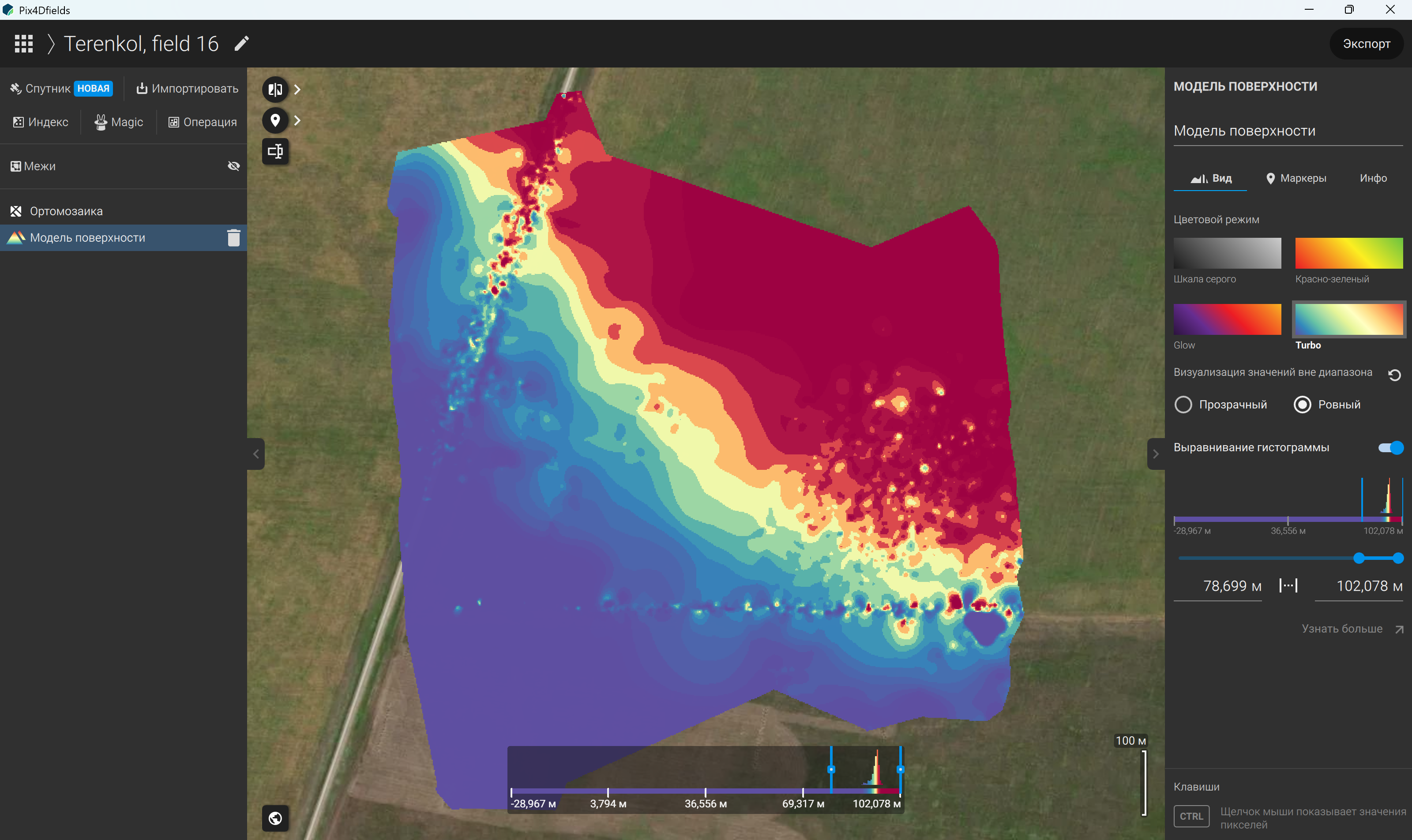
Figure 66 – Applying histogram equalisation to the surface model

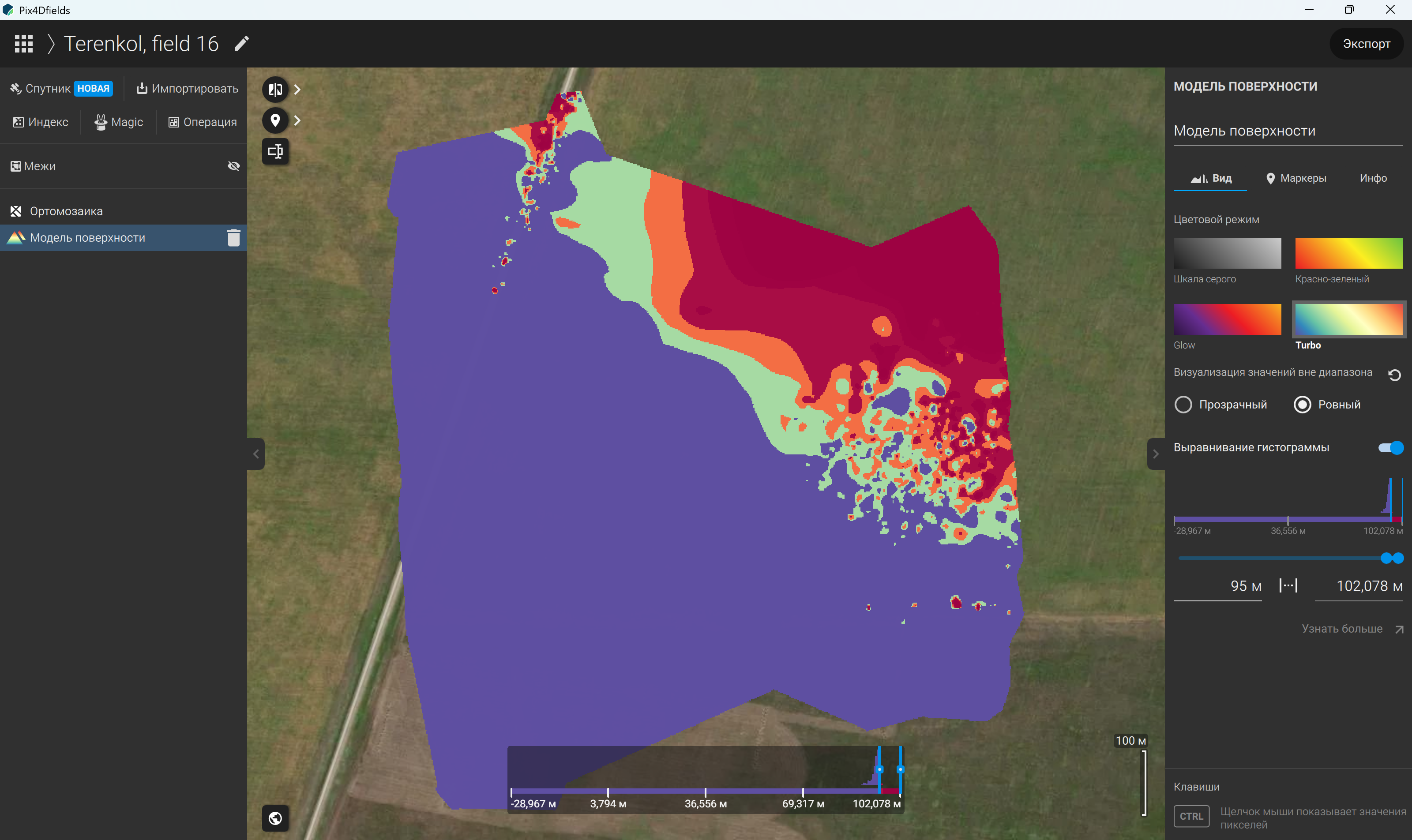
Figure 67 – Manually adjusting the elevation histogram parameters of the surface model

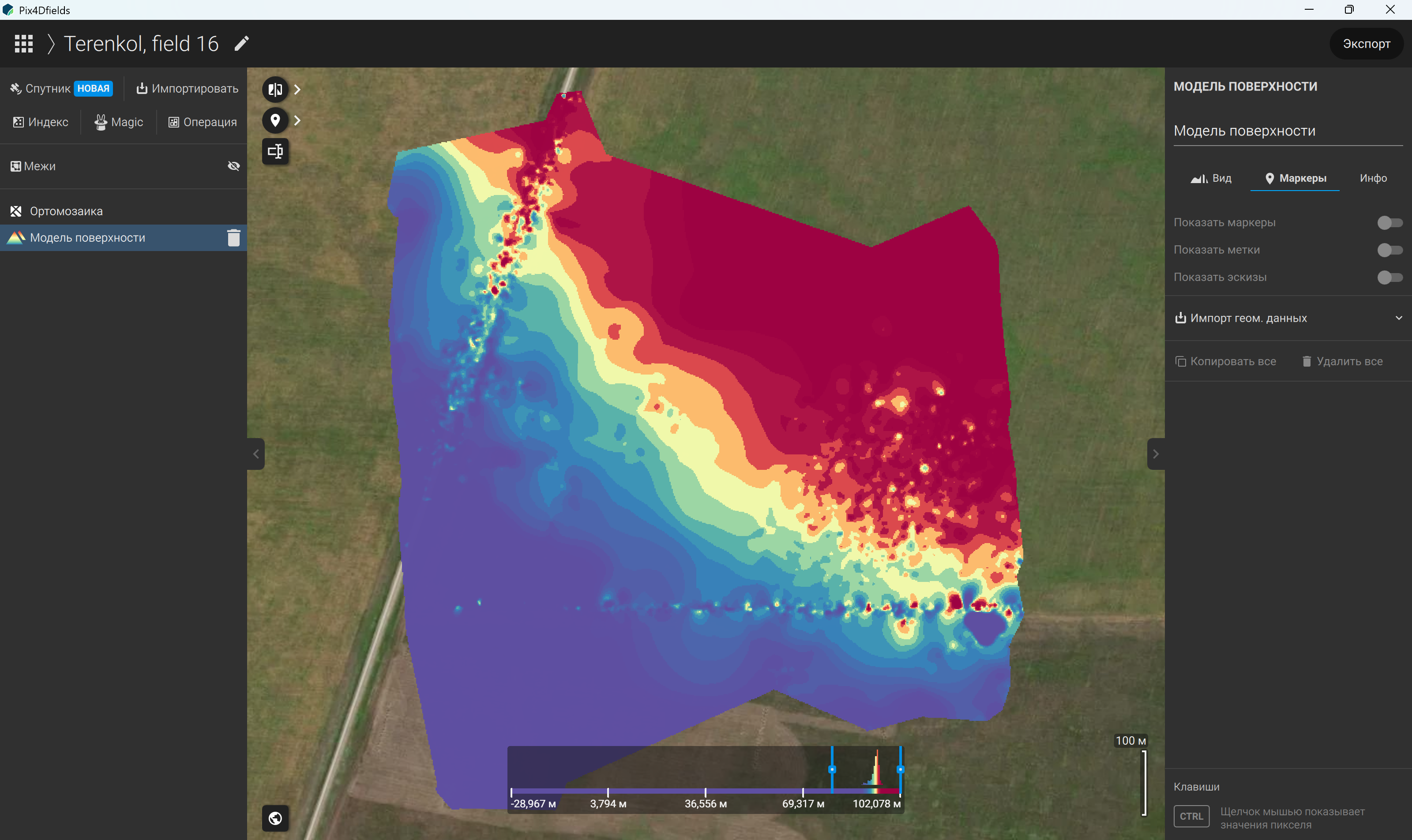
Figure 68 – “Annotations” section of the surface model layer in the right-hand panel

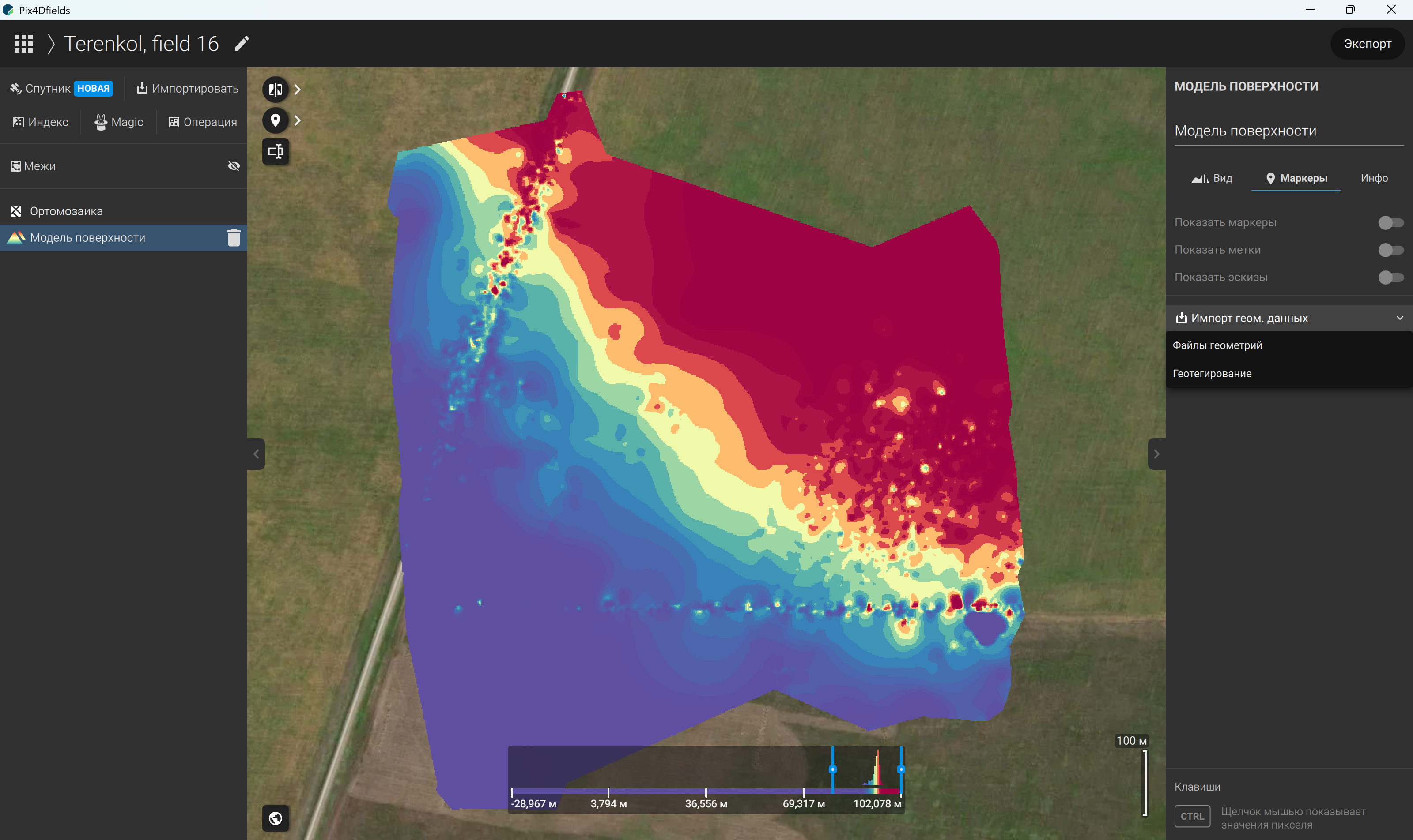
Figure 69 – Importing geometric data through the “Annotations” section of the surface model layer

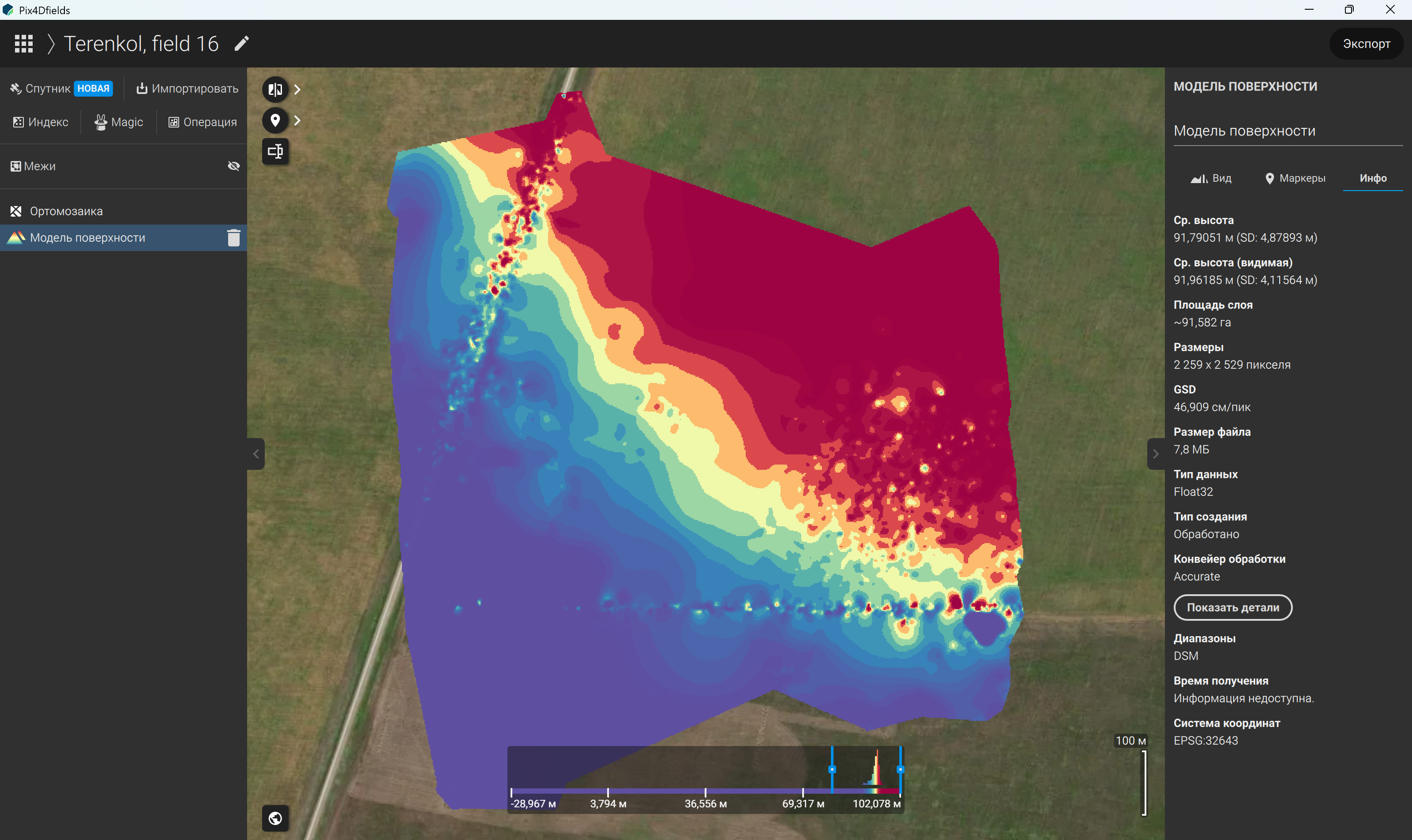
Figure 70 – Information displayed in the “Info” section of the surface model layer

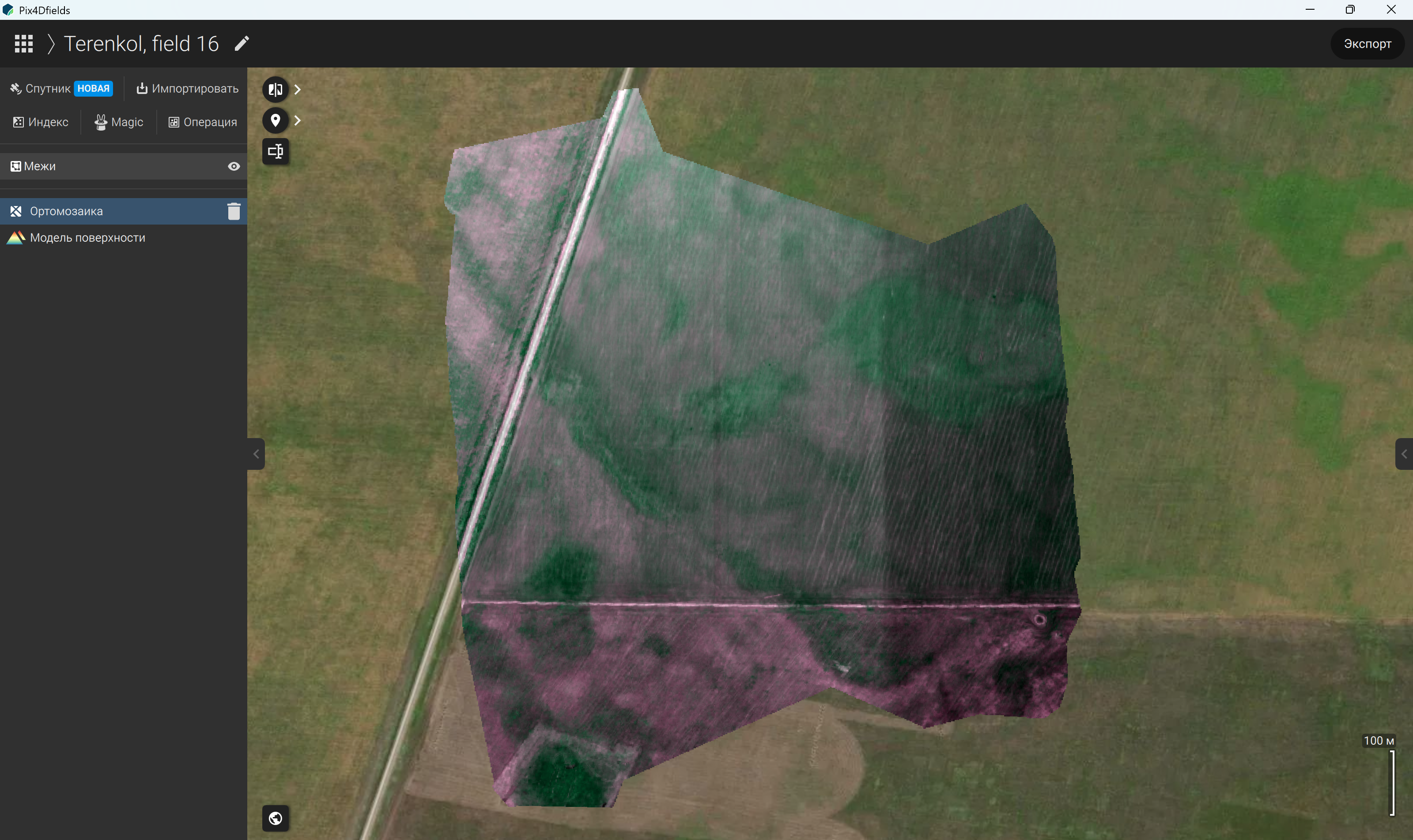
Figure 71 – “Boundaries” tool in the left-hand panel

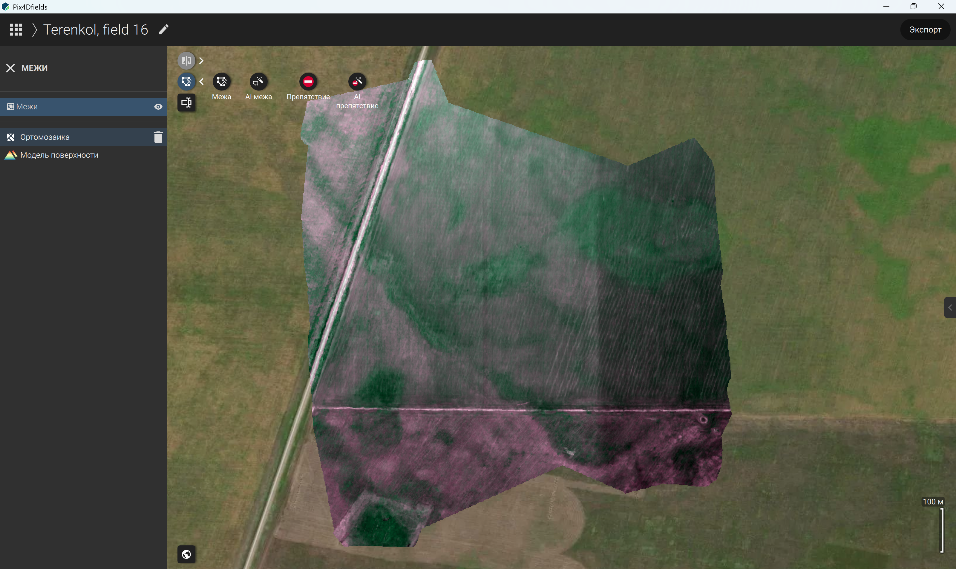
Figure 72 – Available options in the “Boundaries” tool

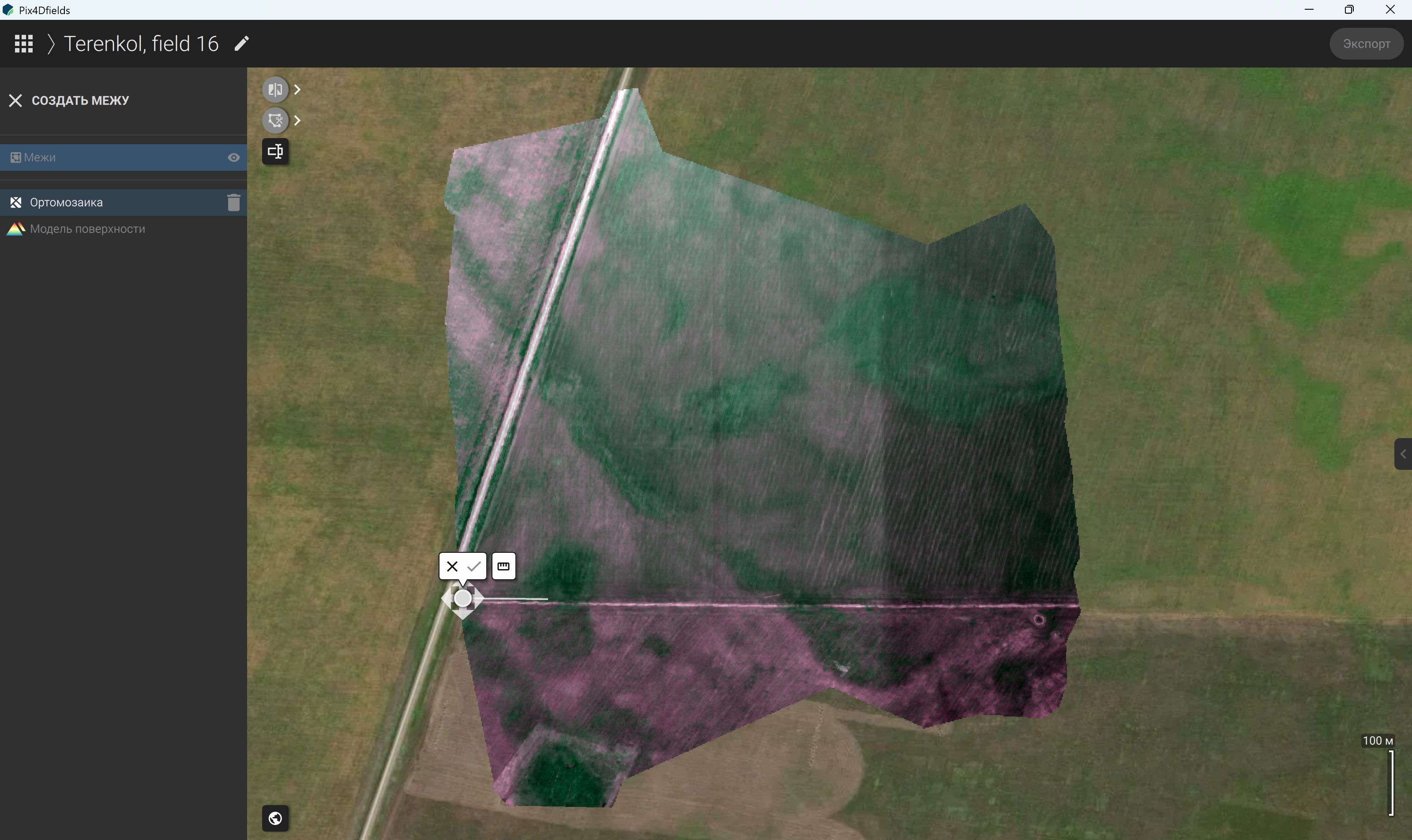
Figure 73 – Defining the starting point for field boundary delineation

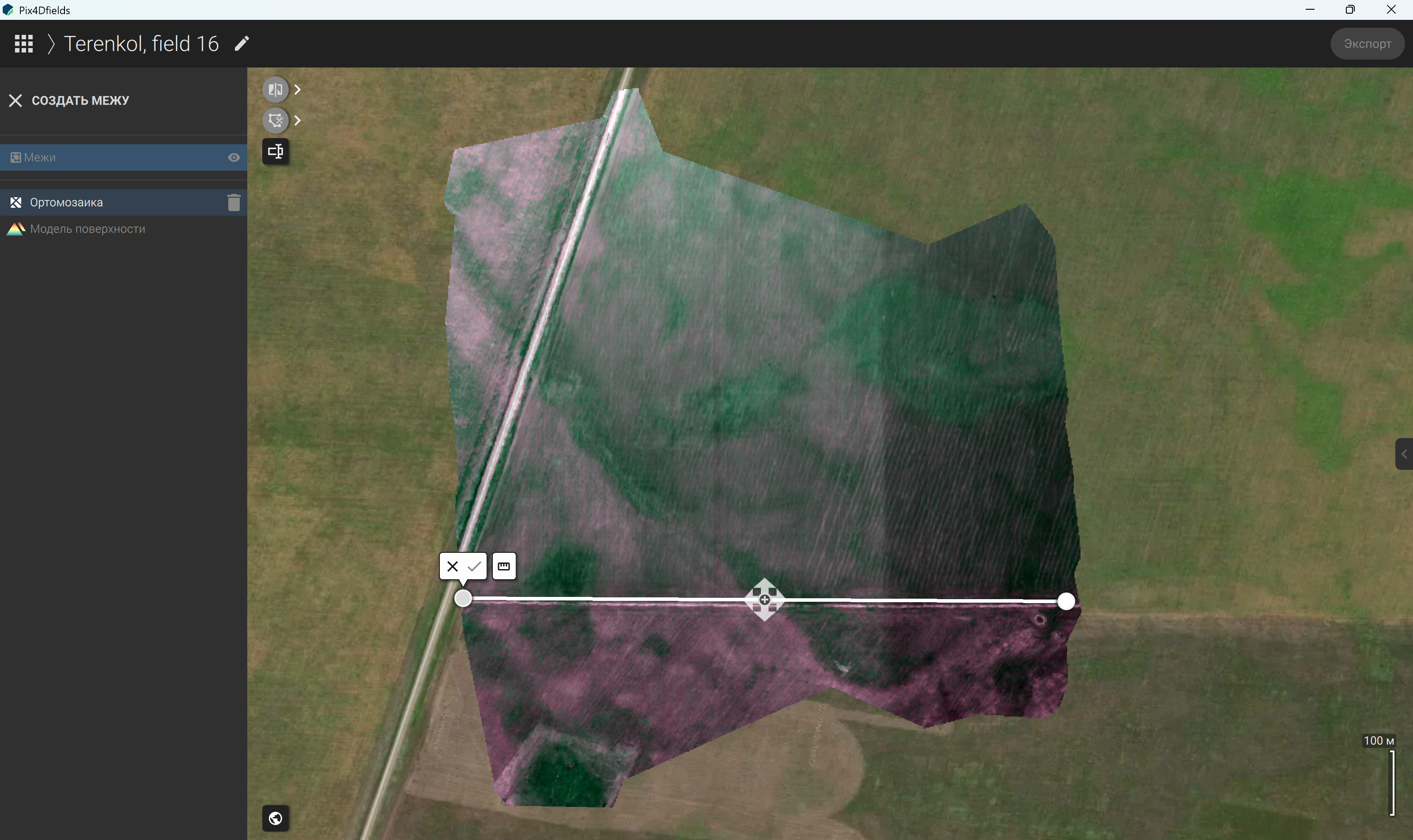
Figure 74 – Tracing one side of the field boundary

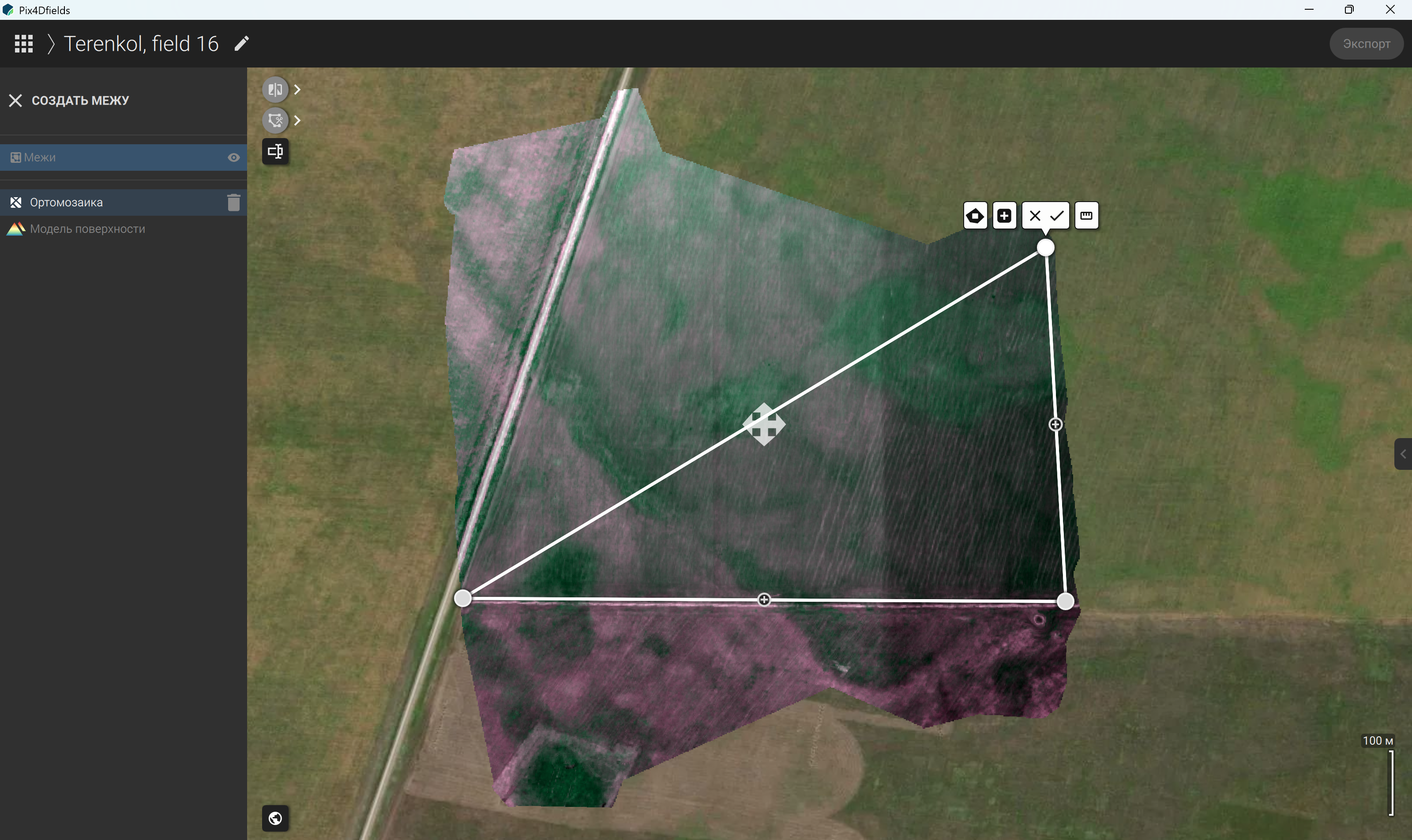
Figure 75 – Selecting the field area

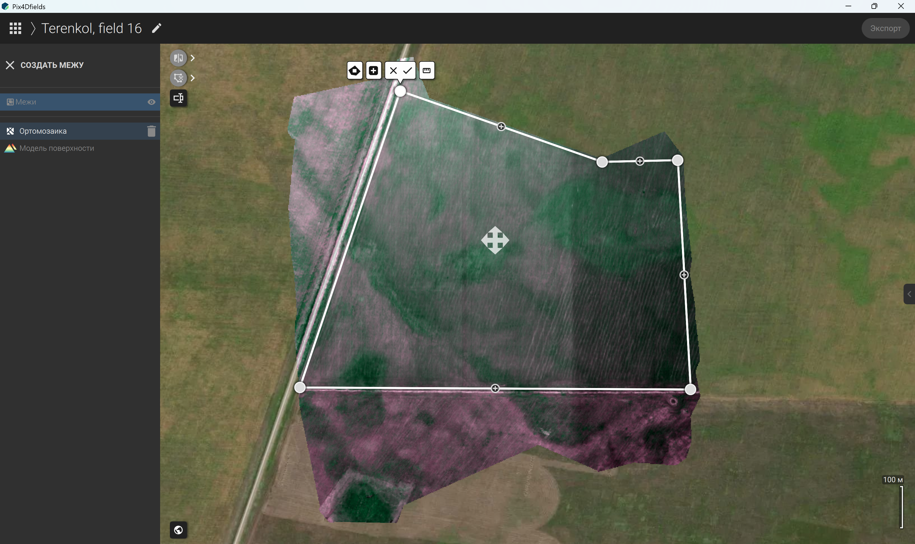
Figure 76 – Delineating the field boundary

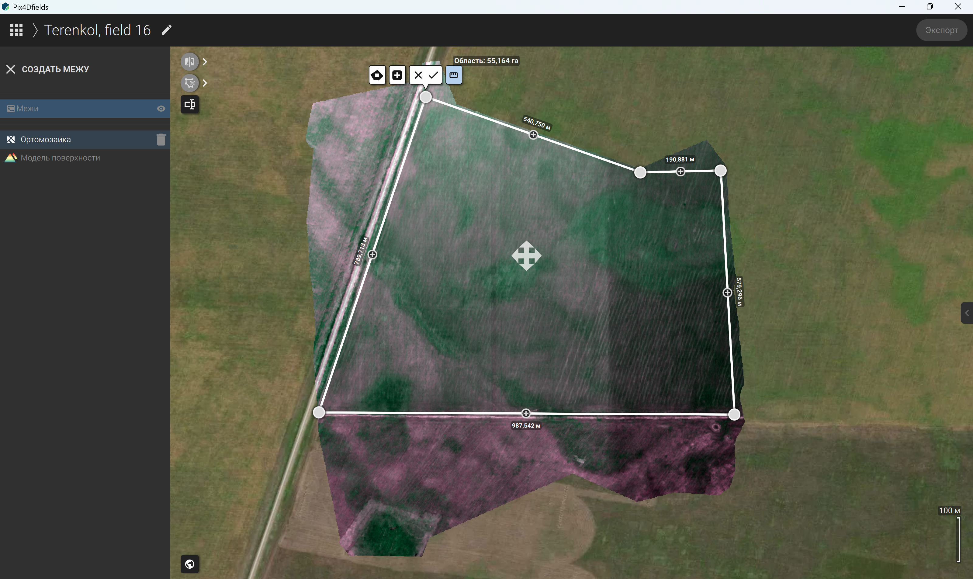
Figure 77 – Measuring the delineated field boundary

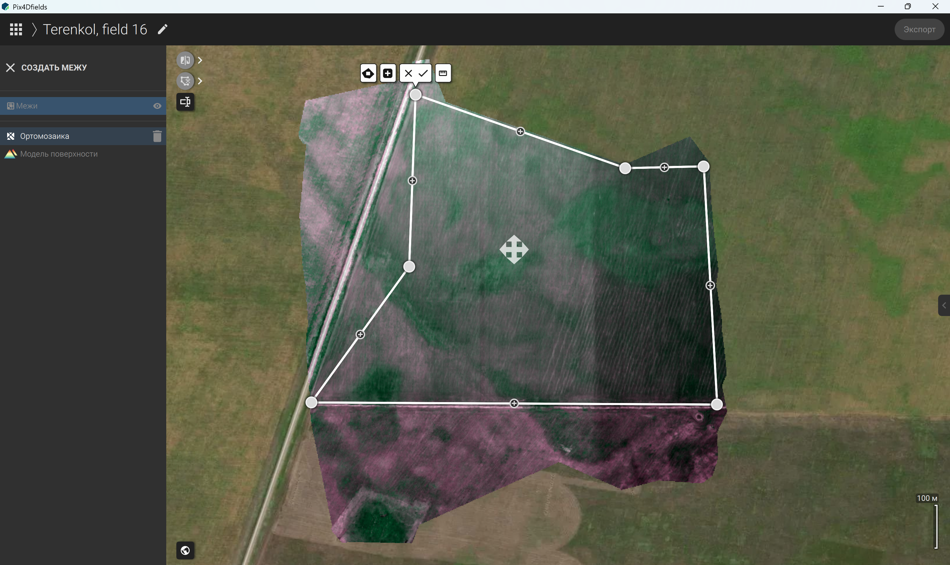
Figure 78 – Editing the delineated field boundary

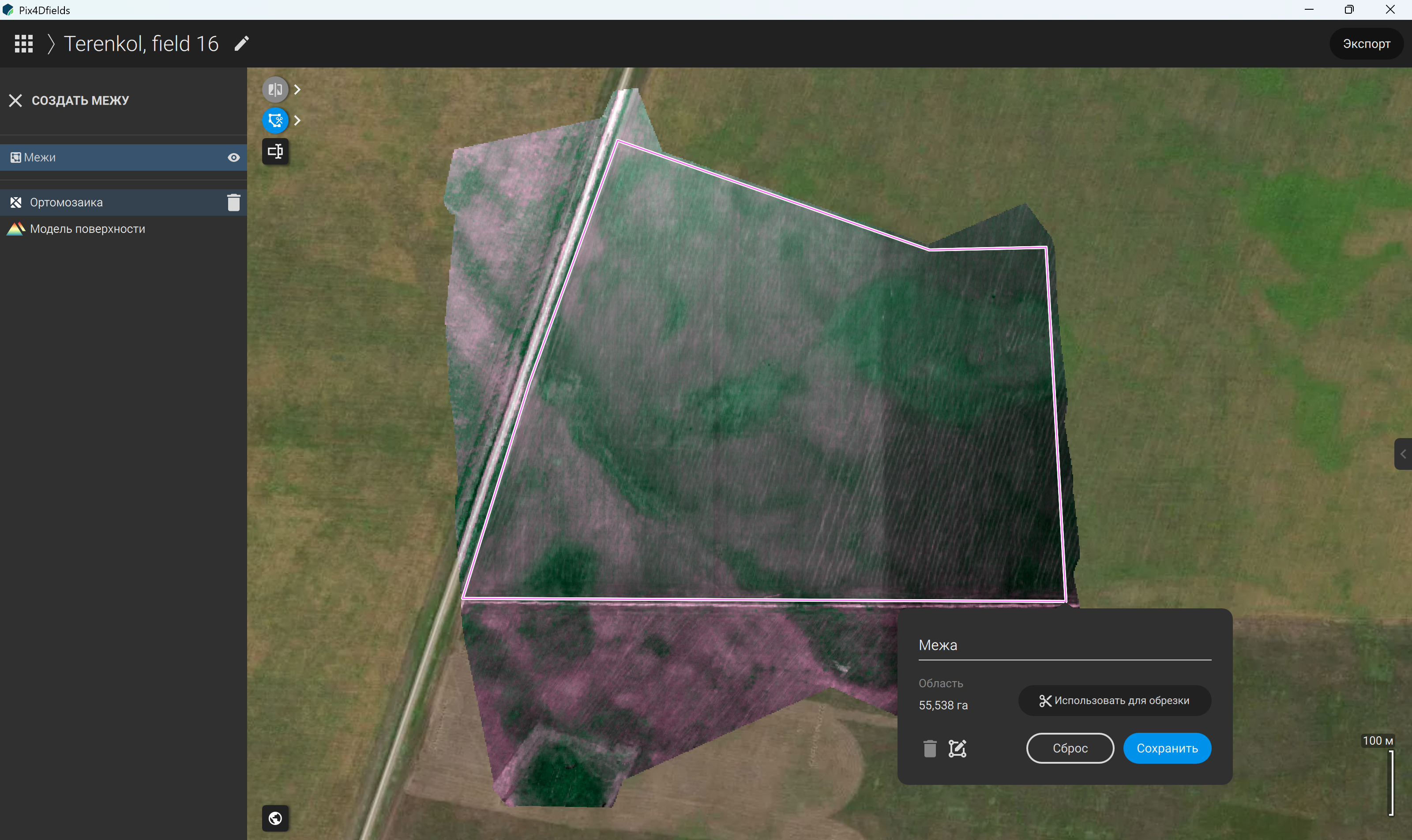
Figure 79 – Generating a field boundary from the selected area

Figure 80 – Saving the delineated field boundary

Figure 81 – Displaying the generated field boundary

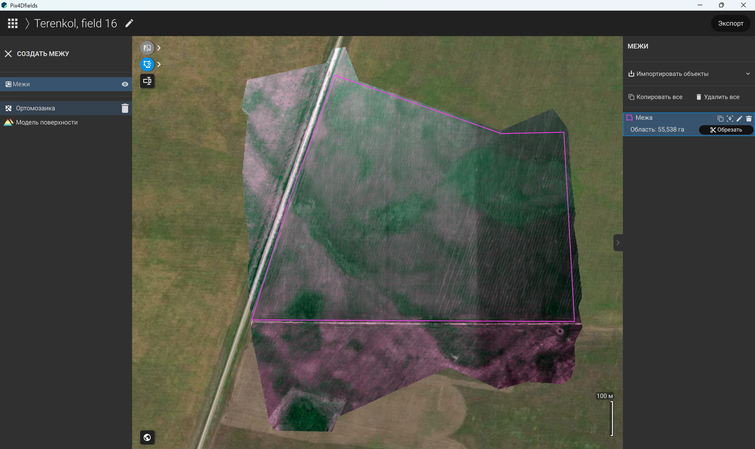
Figure 82 – Restricting the orthomosaic area to the generated field boundary

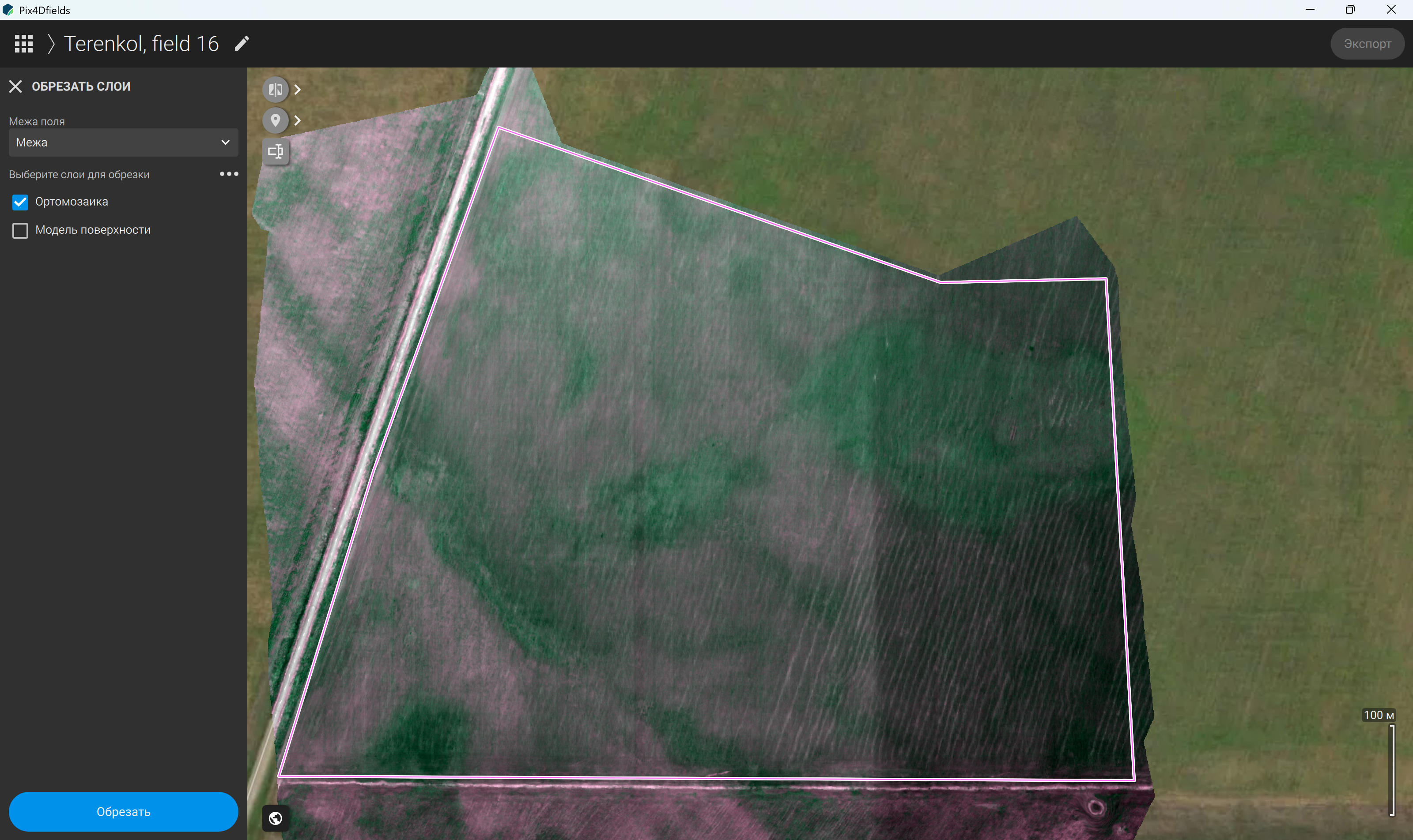
Figure 83 – Selecting the orthomosaic area within the field boundary

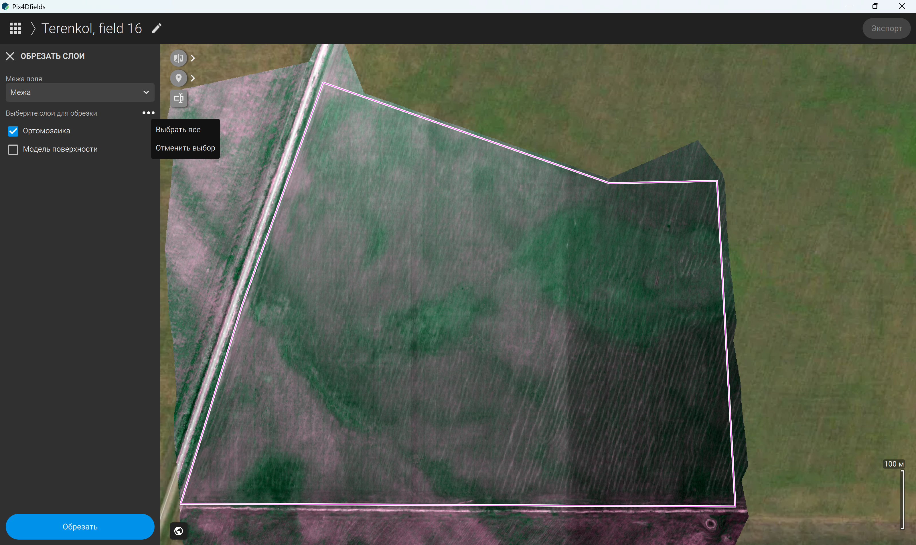
Figure 84 – Applying the selected area to multiple layers simultaneously

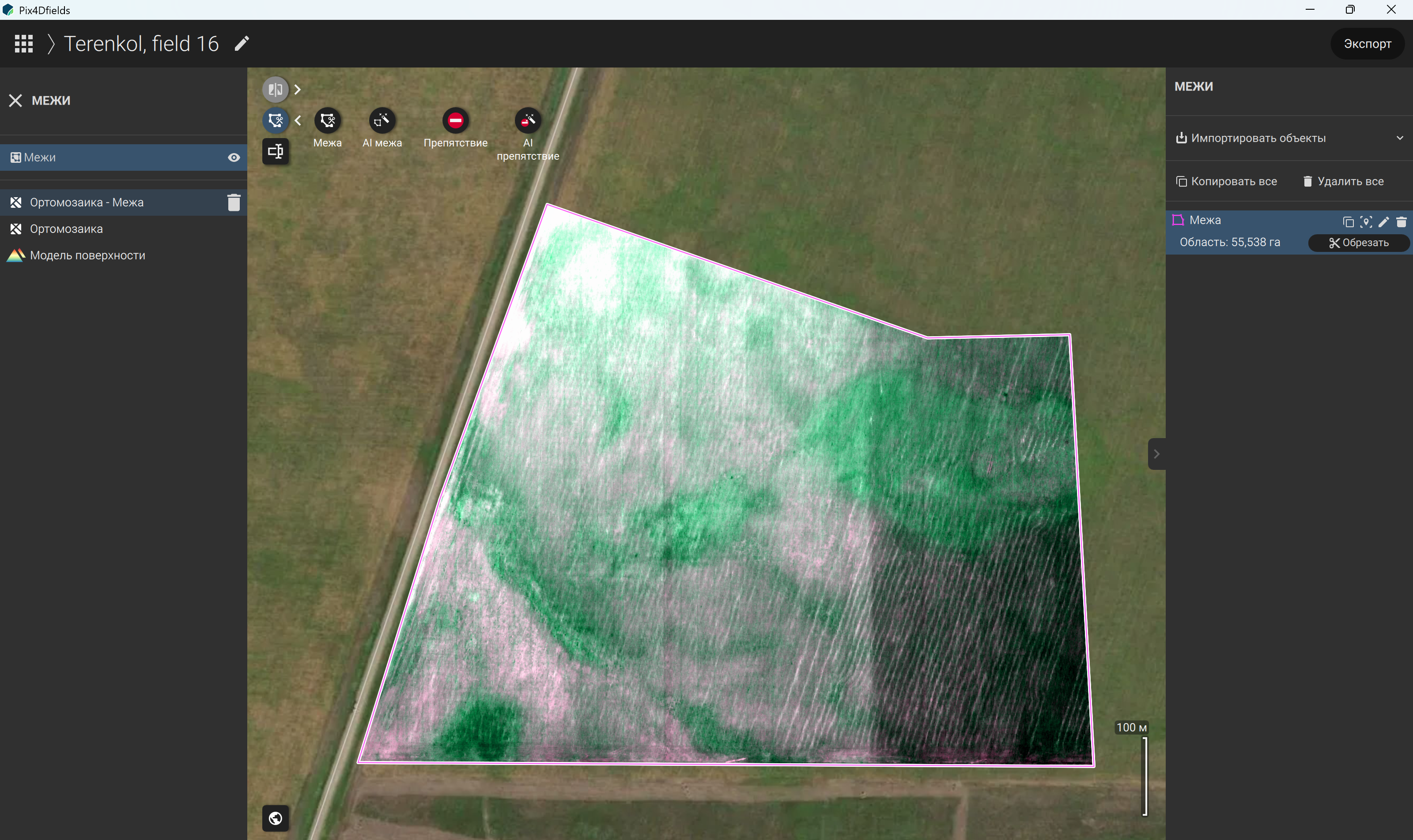
Figure 85 – Resulting orthomosaic boundary

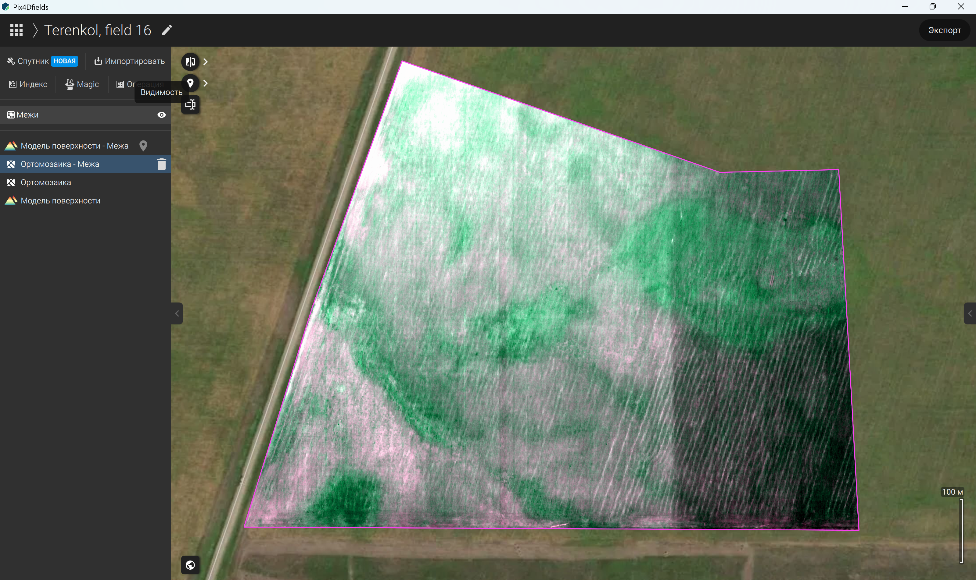
Figure 86 – Displaying the field boundary on the map

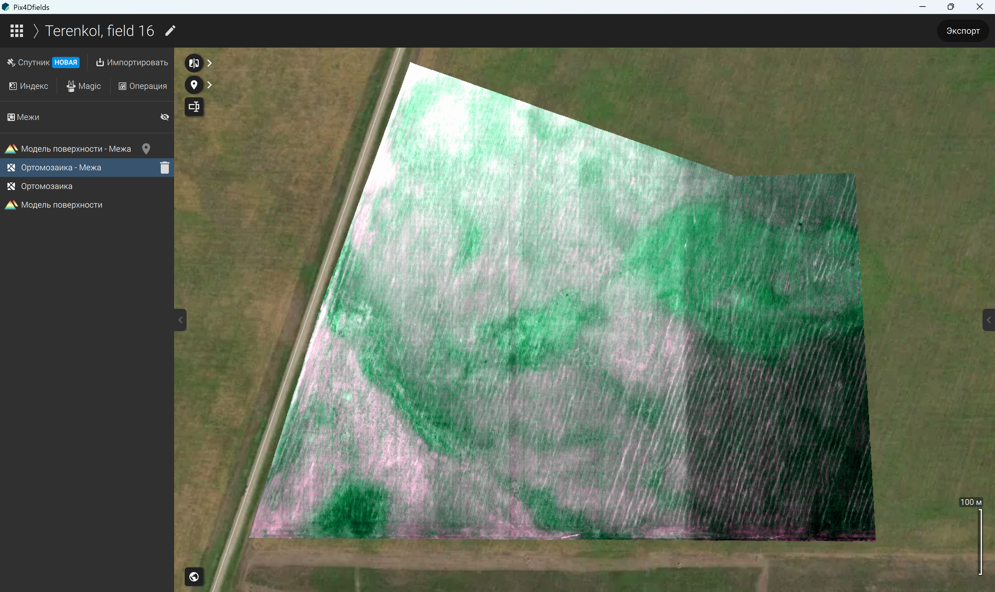
Figure 87 – Viewing the map with the field boundary hidden

The delineated field boundaries can be saved and imported into other projects, allowing the same boundaries to be reused when processing new survey data for the same area. If a boundary has been created on the orthomosaic, it can subsequently be transferred to the surface model through a series of operations: projecting the boundary onto the surface model (Figure 88), overlaying it on the target layer (Figure 89), and clipping (cropping) the layer to the defined boundary (Figure 90). As a result, the field boundary is applied to the corresponding layer (Figure 91). Its visibility can be toggled using the eye icon in the “Boundaries” tool.

Three buttons are located in the upper-left corner of the map interface (Figure 92). The first provides access to map comparison tools, which support two display modes. The “Split” mode displays two maps side by side, allowing the user to compare different layers, such as the surface model and the orthomosaic (Figure 93). The “Composite” mode combines two maps within a single view, facilitating the visual comparison and joint analysis of different layers (Figure 94). The second button provides access to annotation tools (Figure 95). Annotations can be created in several geometric forms, including points (Figures 96, 97), line segments (Figures 98, 99), lines (Figures 100, 101), and polygons (Figures 102-104). An AI-assisted tool may also be available for delineating selected areas. During annotation, a panel appears at the bottom of the screen, displaying the relevant tool settings and available keyboard shortcuts. The third button allows users to navigate directly to a specified location by entering a place name or GPS coordinates (Figures 105, 106).

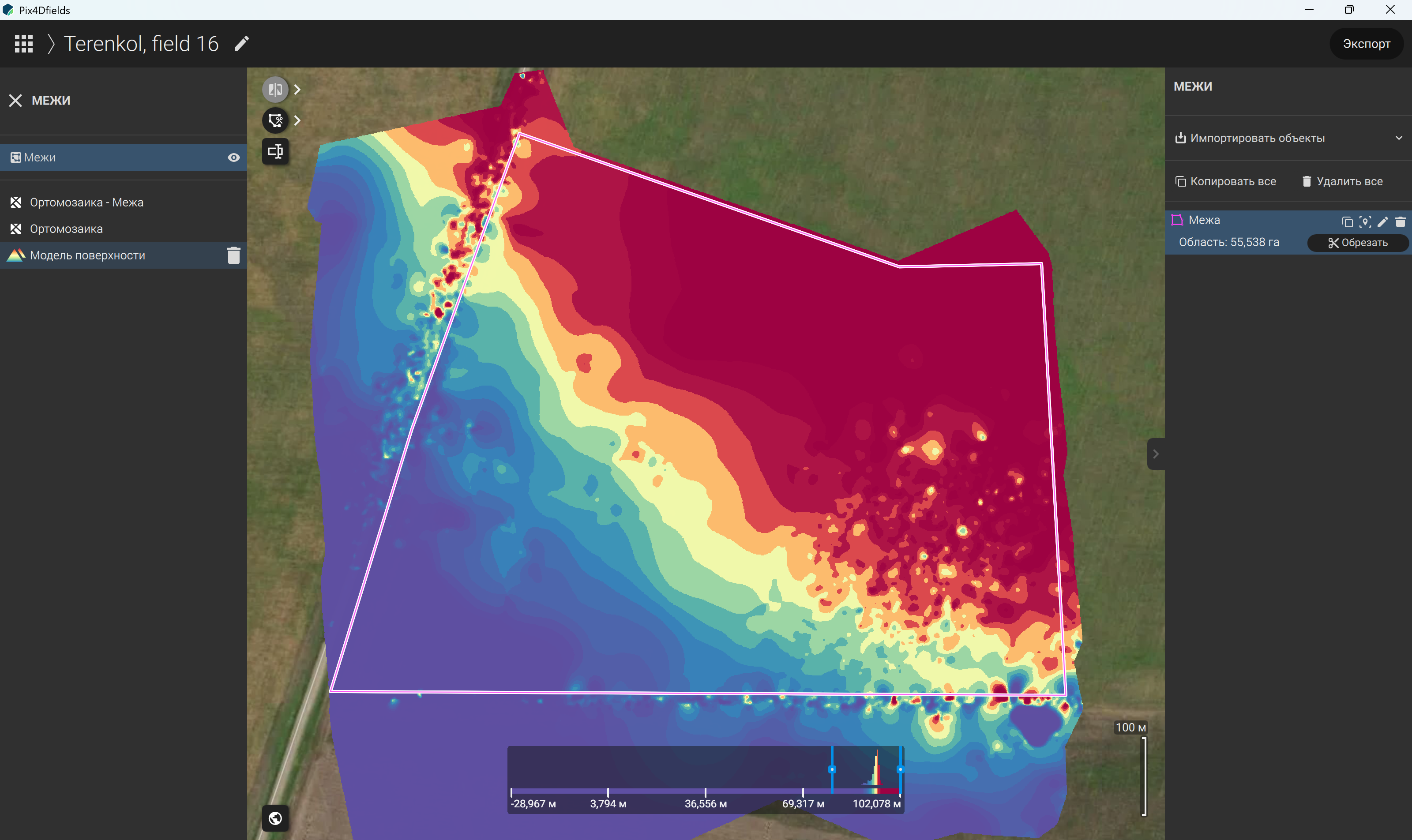
Figure 88 – Projecting the generated field boundary onto the surface model

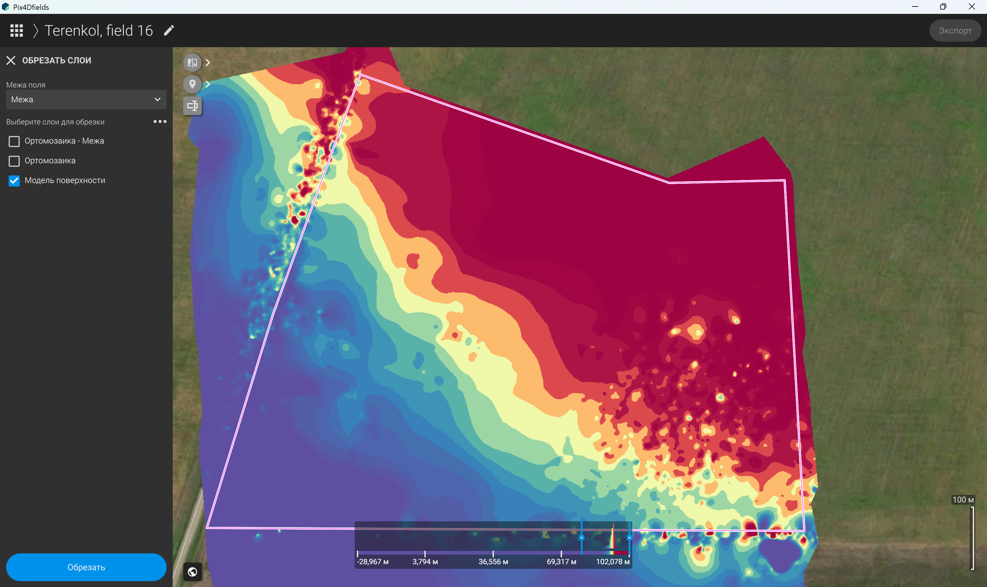
Figure 89 – Overlaying the generated field boundary on the surface model

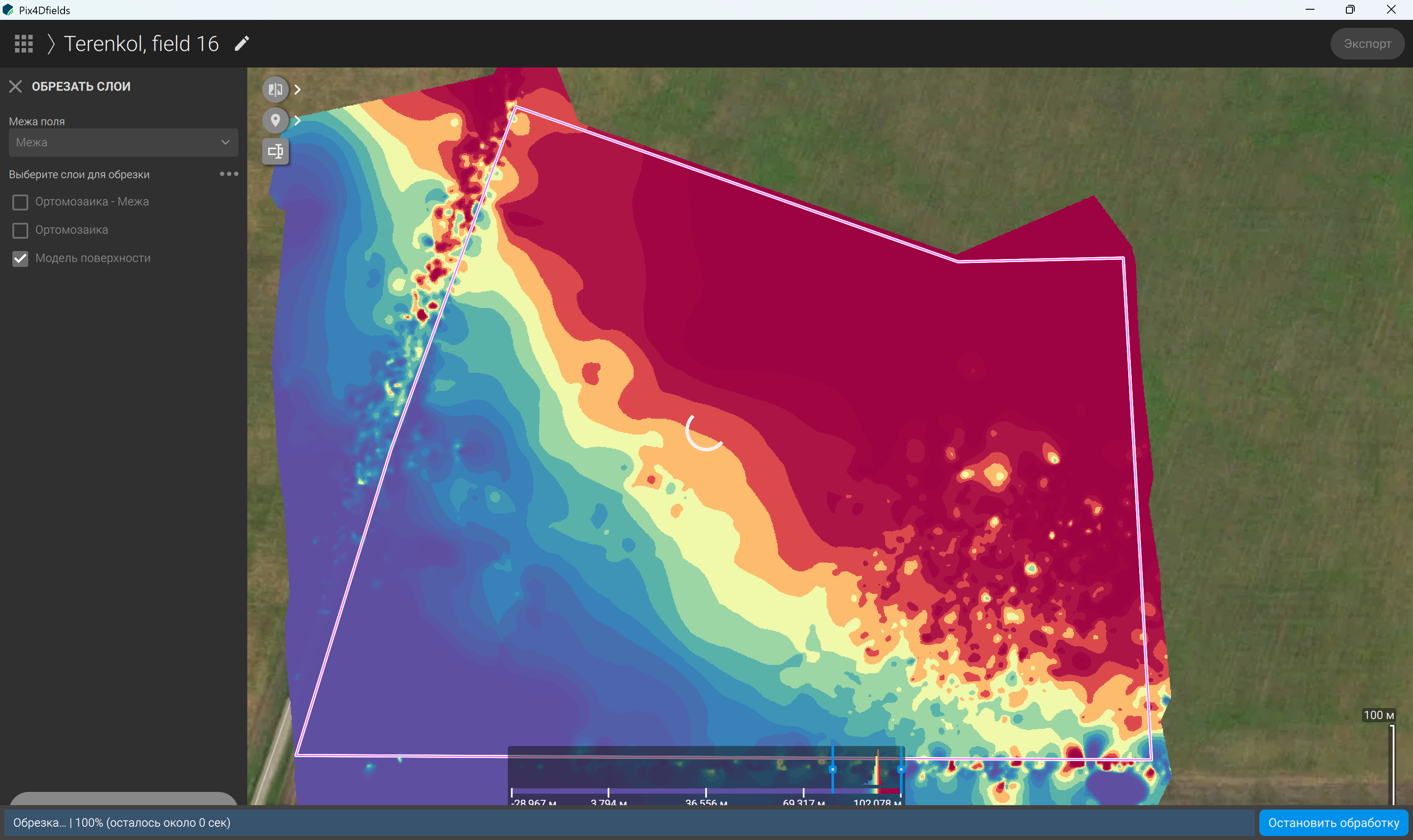
Figure 90 – Clipping (cropping) the surface model to the generated field boundary

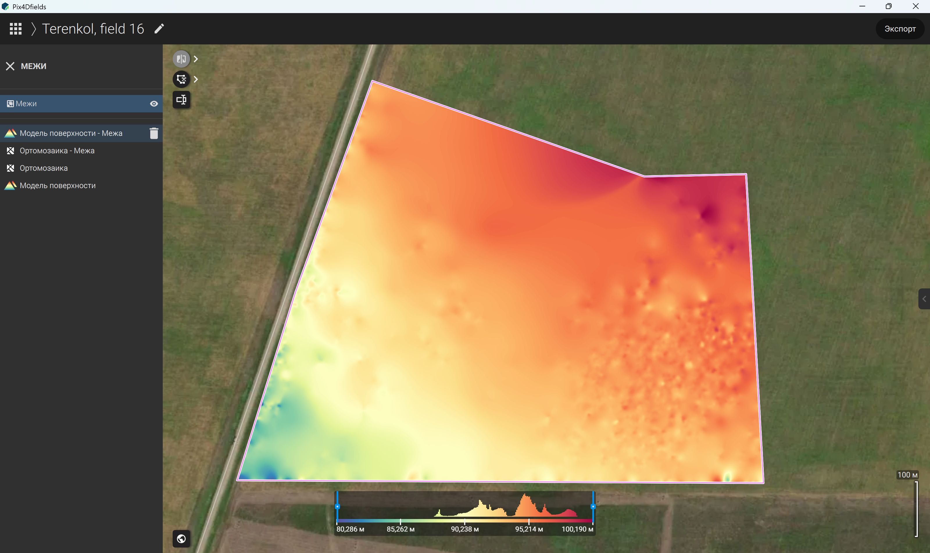
Figure 91 – Surface model clipped to the field boundary

The upper section of the left-hand panel contains the main data processing tools (Figure 107). These tools allow users to import satellite imagery and supplementary images (Figure 108), process the available data, and calculate spectral indices. The “Operation” tool provides a guided workflow for processing map data according to the intended analytical objective (Figure 109). The Operations Wizard guides users through the required configuration stages, offers options for generating new layers, and provides access to relevant reference information. The workflow varies depending on the selected operation. The available configurations illustrated in this study include processing without pre-filling grid cells (Figure 110), pre-filling the grid based on an annotation (Figure 111), pre-filling the grid using an index layer for zoning (Figure 112), and pre-filling the grid using reference cells from the orthomosaic with the Magic Tool (Figure 113).

The Magic Tool supports guided map processing based on the selected analytical objective (Figure 114). Its operation involves selecting the relevant field boundaries (Figure 115), choosing a source layer, and identifying obstacles that may affect the processing results (Figure 116). Any suitable project layer can be selected as the source, depending on the intended task. Where necessary, obstacles such as trees, water bodies, and other features can be marked to account for them during subsequent processing. Grid parameters can also be configured manually using the Magic Tool (Figure 117).

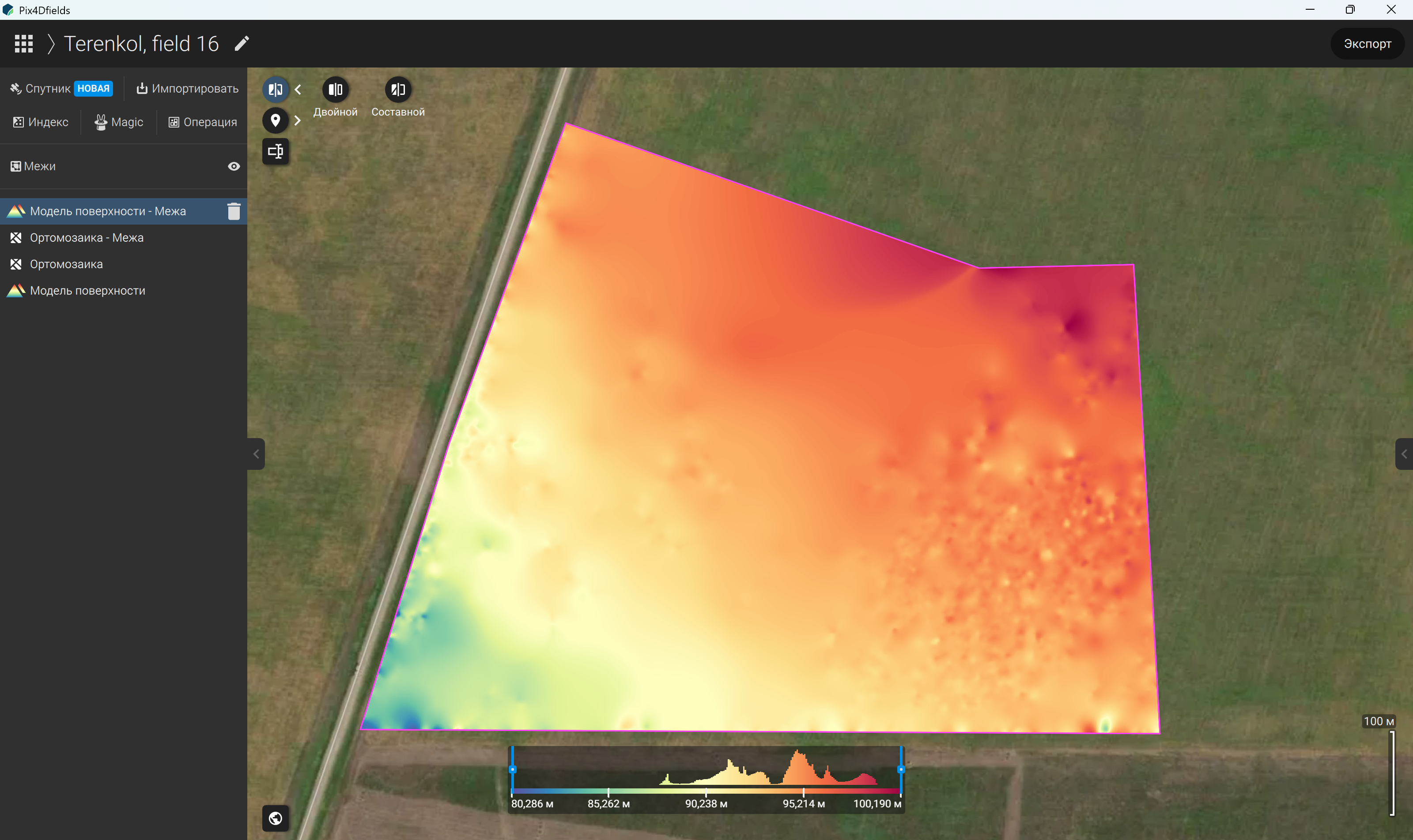
Figure 92 – Map navigation and comparison tools

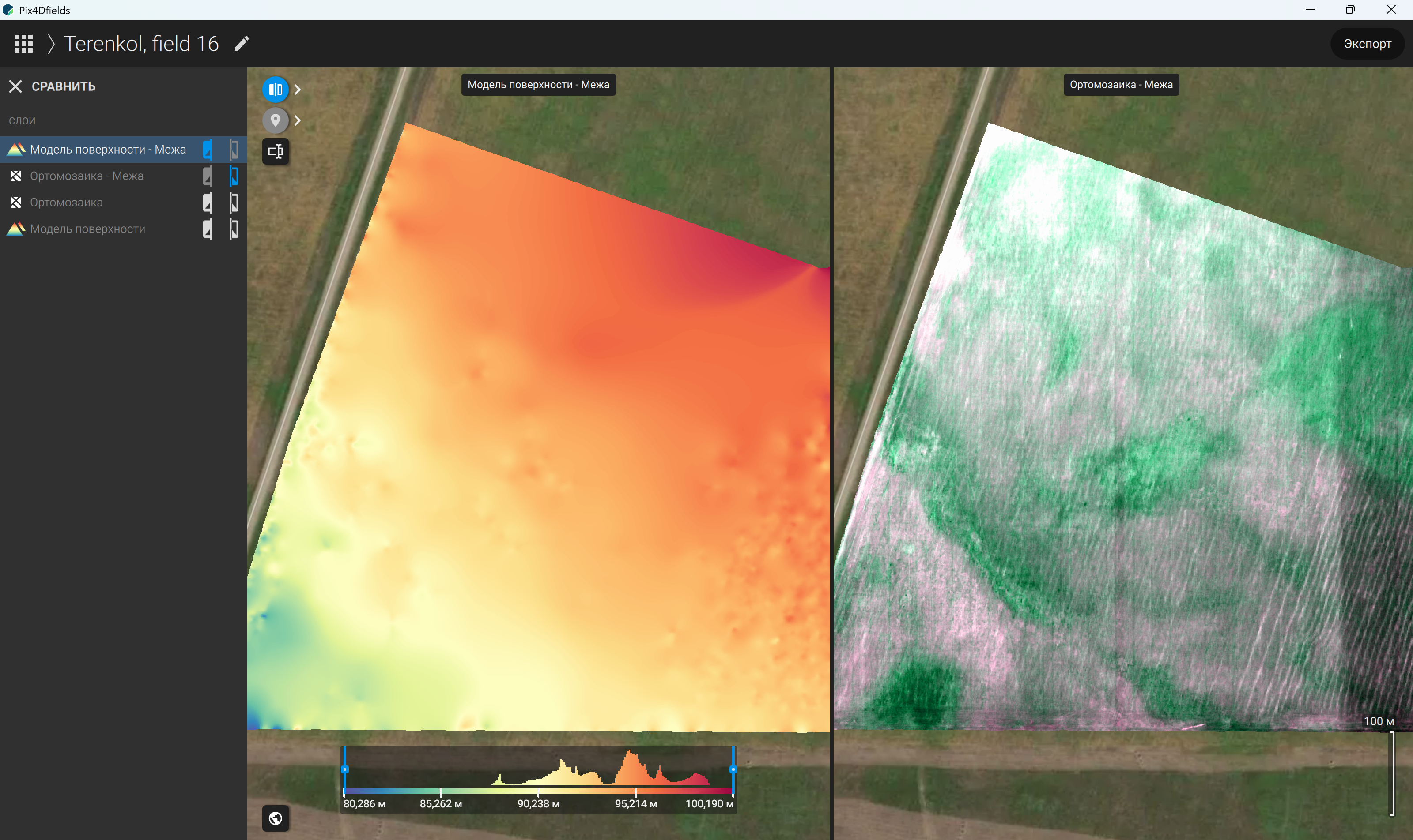
Figure 93 – Comparing map layers in “Split” mode

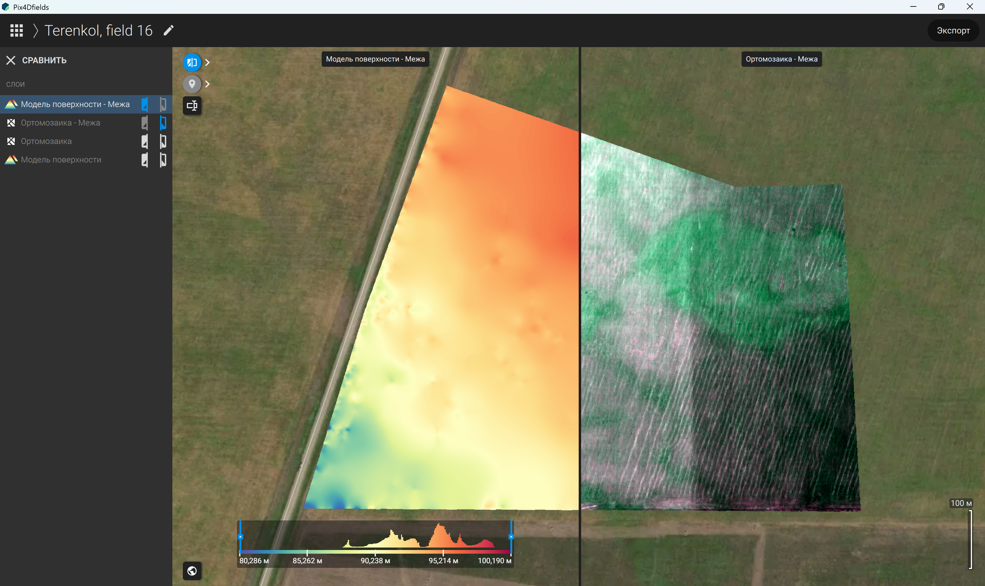
Figure 94 – Comparing map layers in “Composite” mode

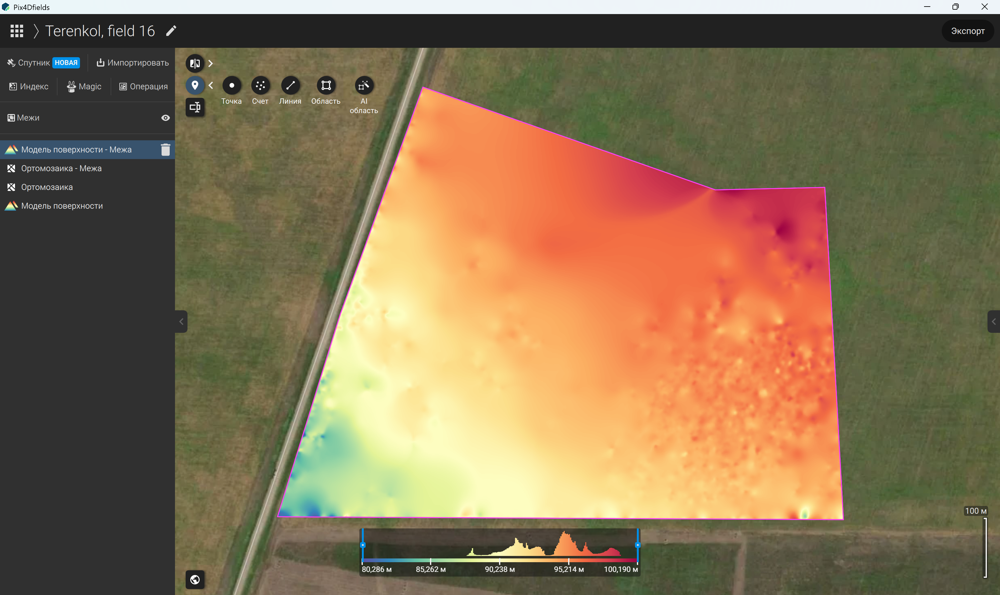
Figure 95 – Annotation tools for marking points and delineating areas on the map

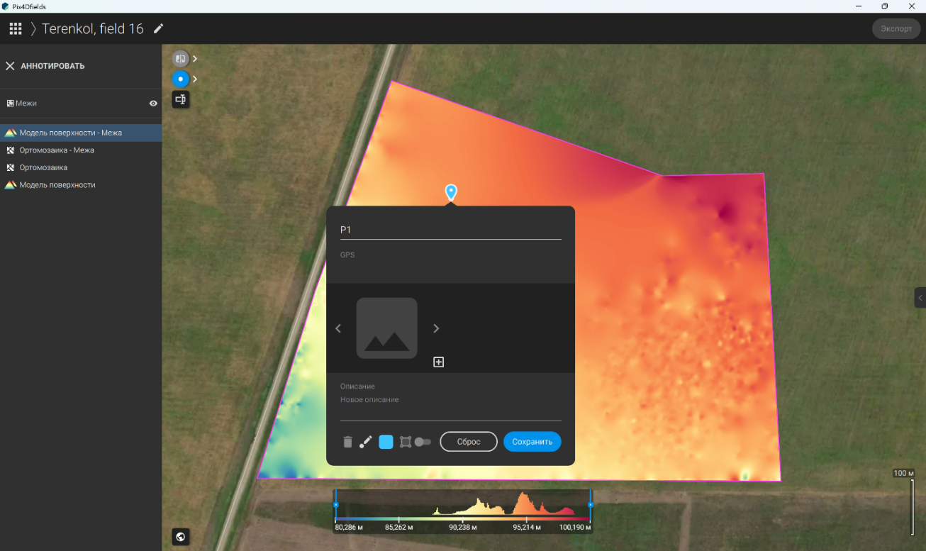
Figure 96 – Placing a point annotation on the map (P1)

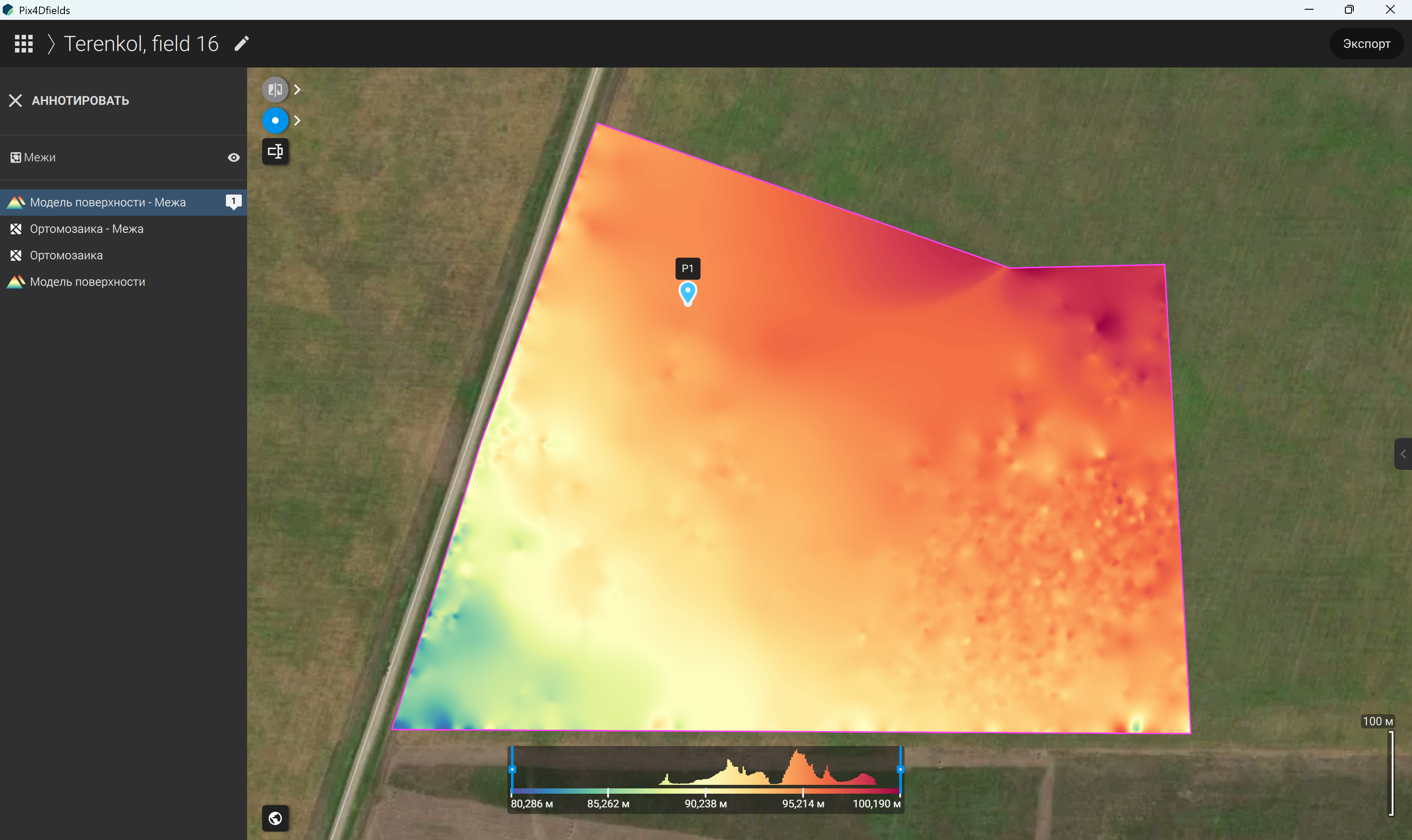
Figure 97 – Displaying the point annotation on the map (P1)

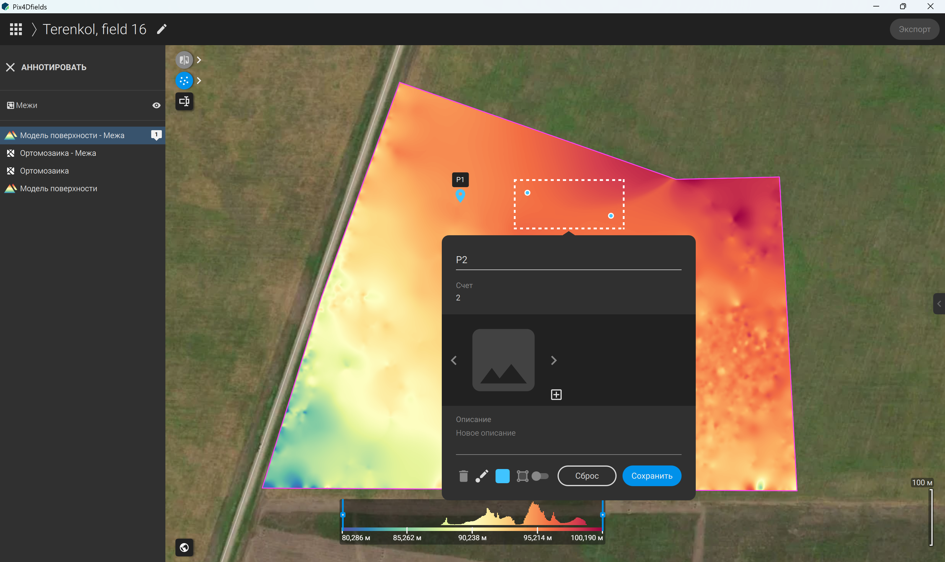
Figure 98 – Placing a line segment annotation on the map (P2)

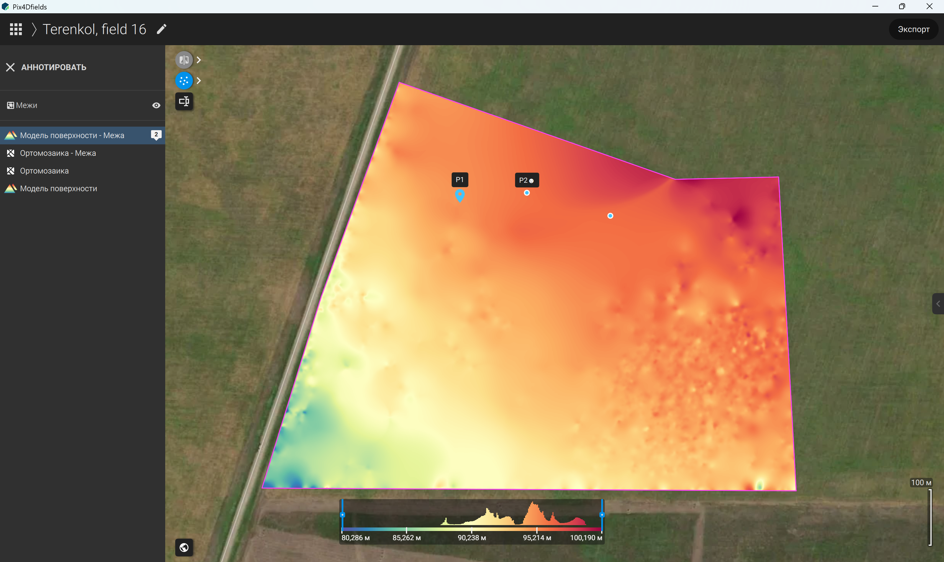
Figure 99 – Displaying the line segment annotation on the map (P2)

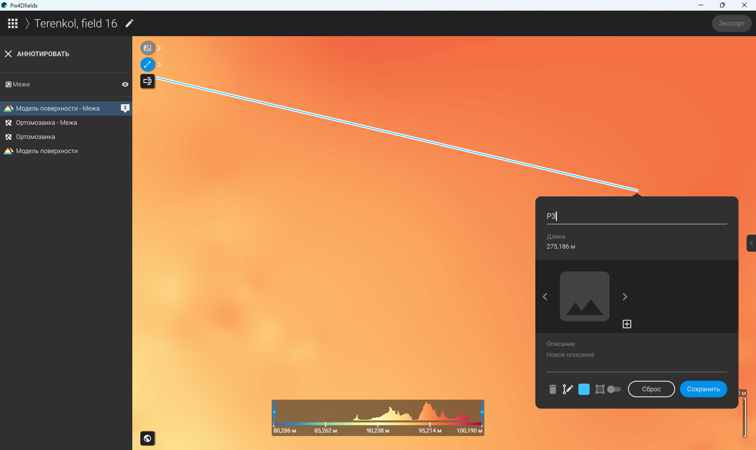
Figure 100 – Drawing a line annotation on the map (P3)

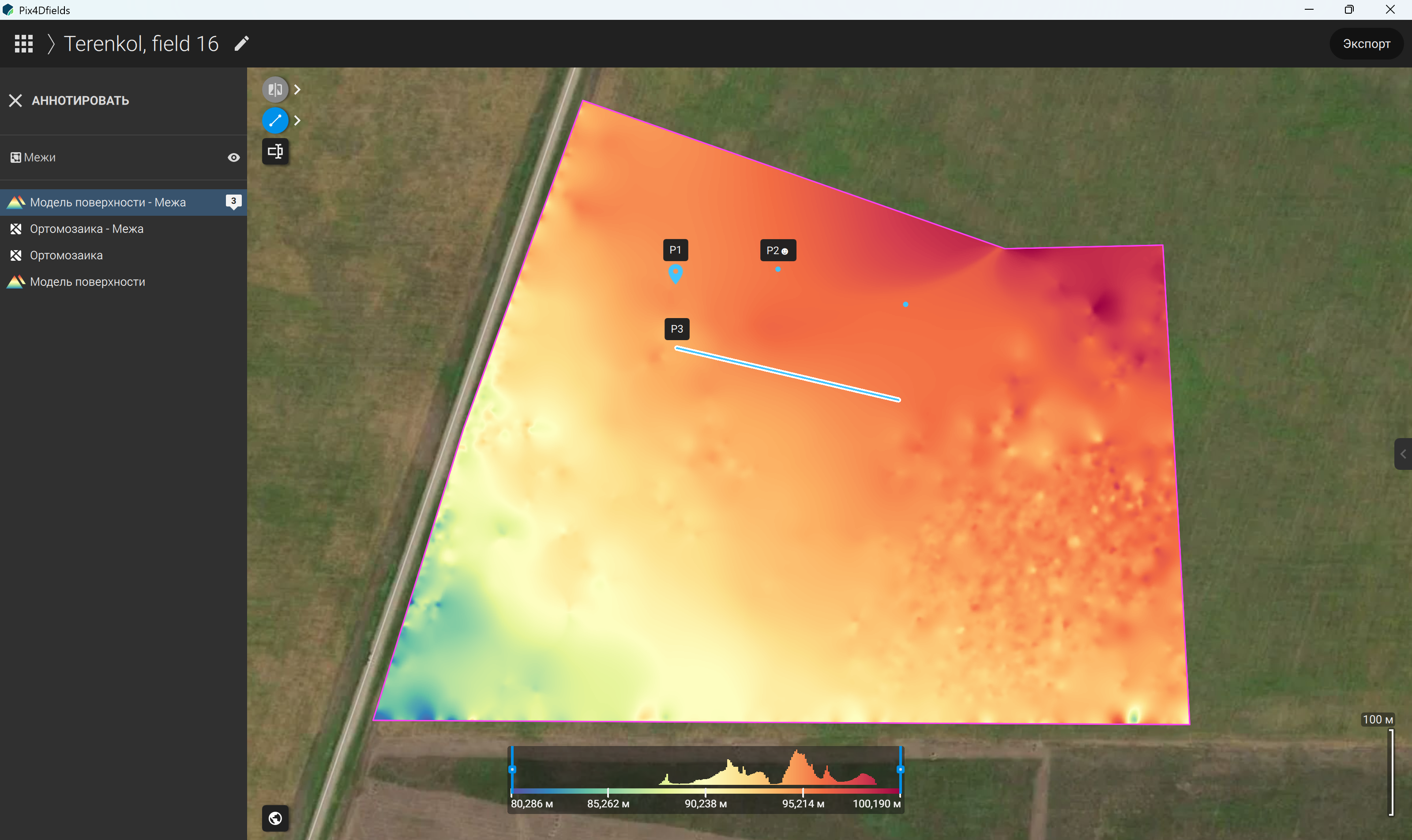
Figure 101 – Displaying the line annotation on the map (P3)

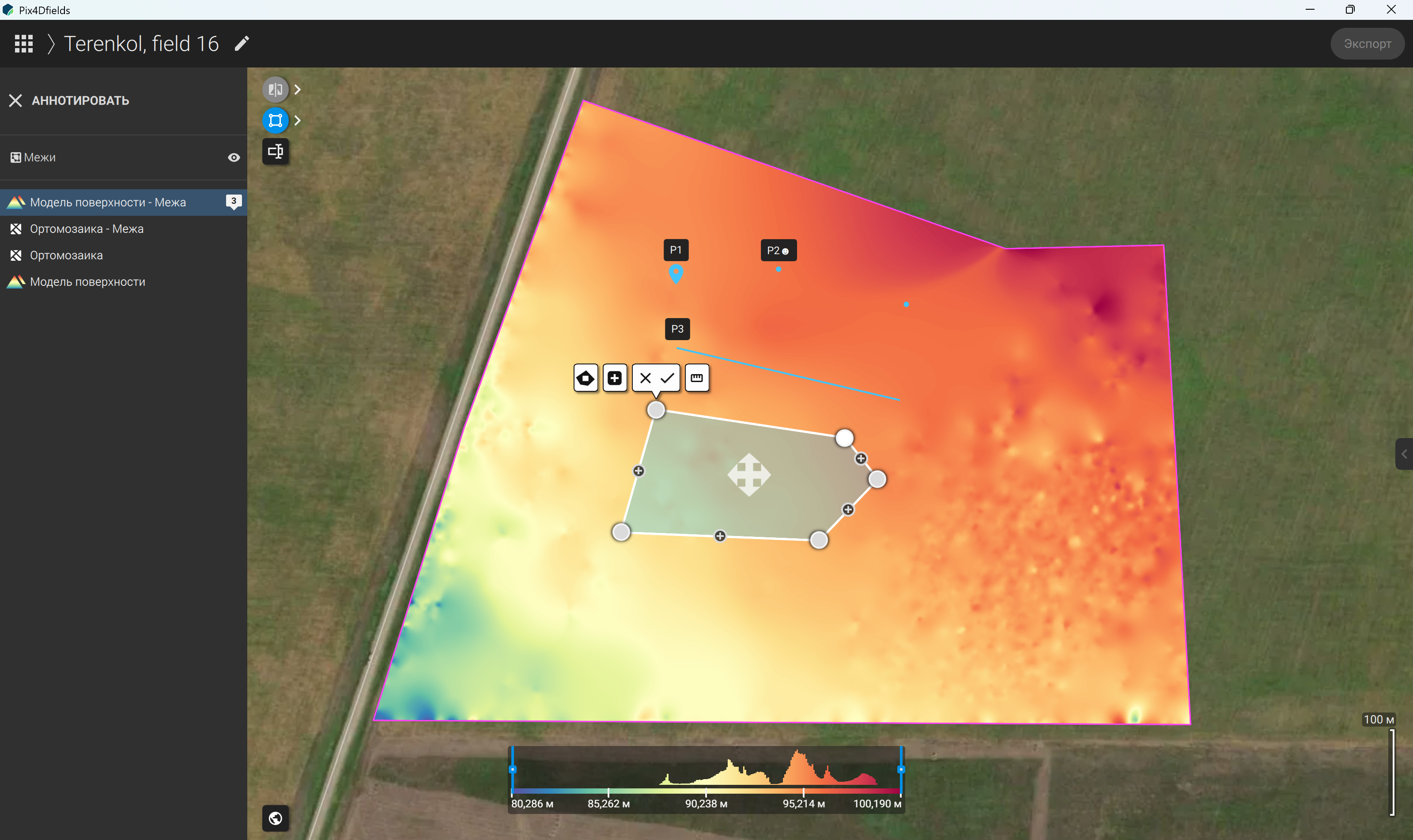
Figure 102 – Delineating a selected area on the map

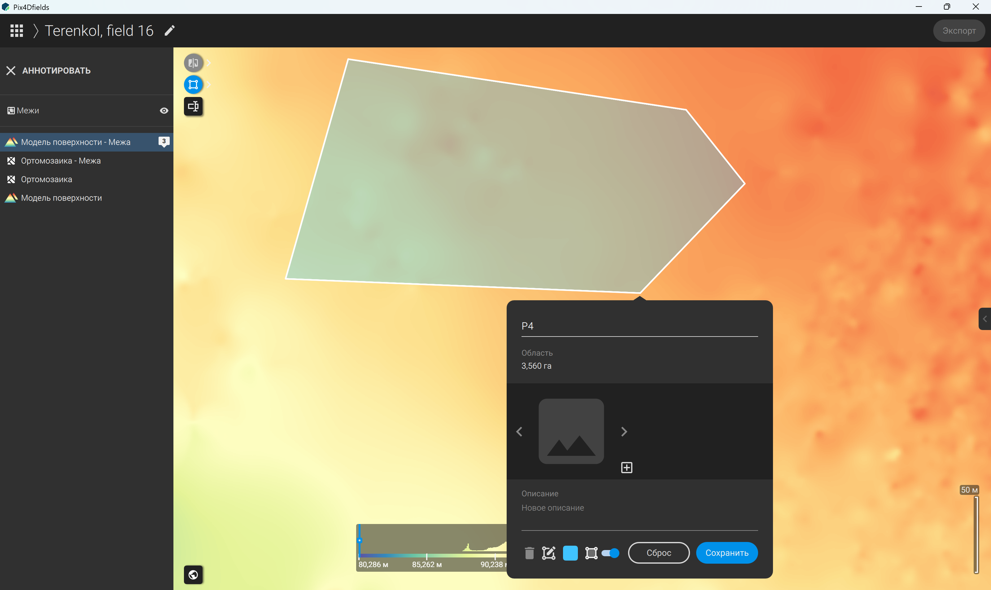
Figure 103 – Creating a polygon annotation on the map (P4)

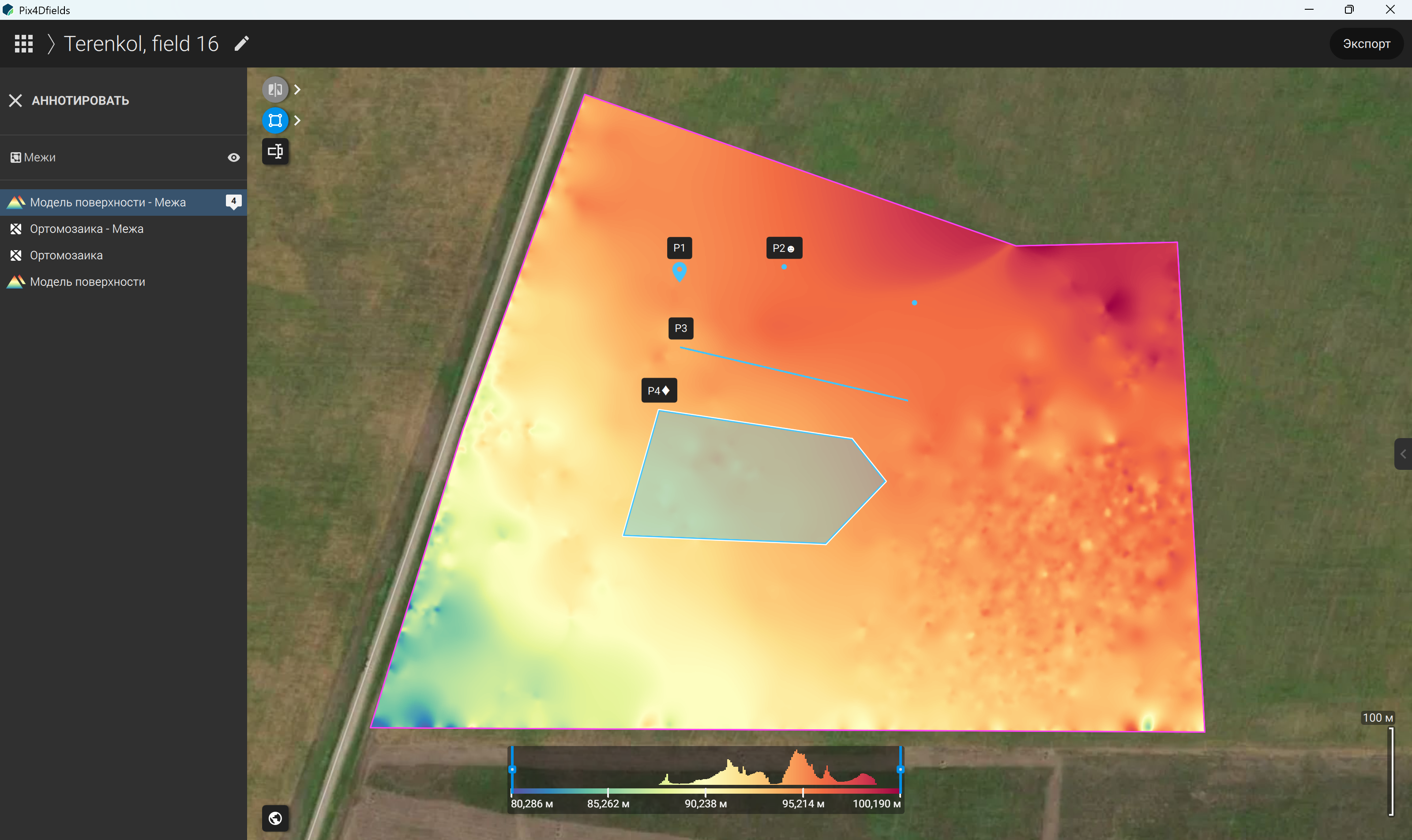
Figure 104 – Displaying the polygon annotation on the map (P4)

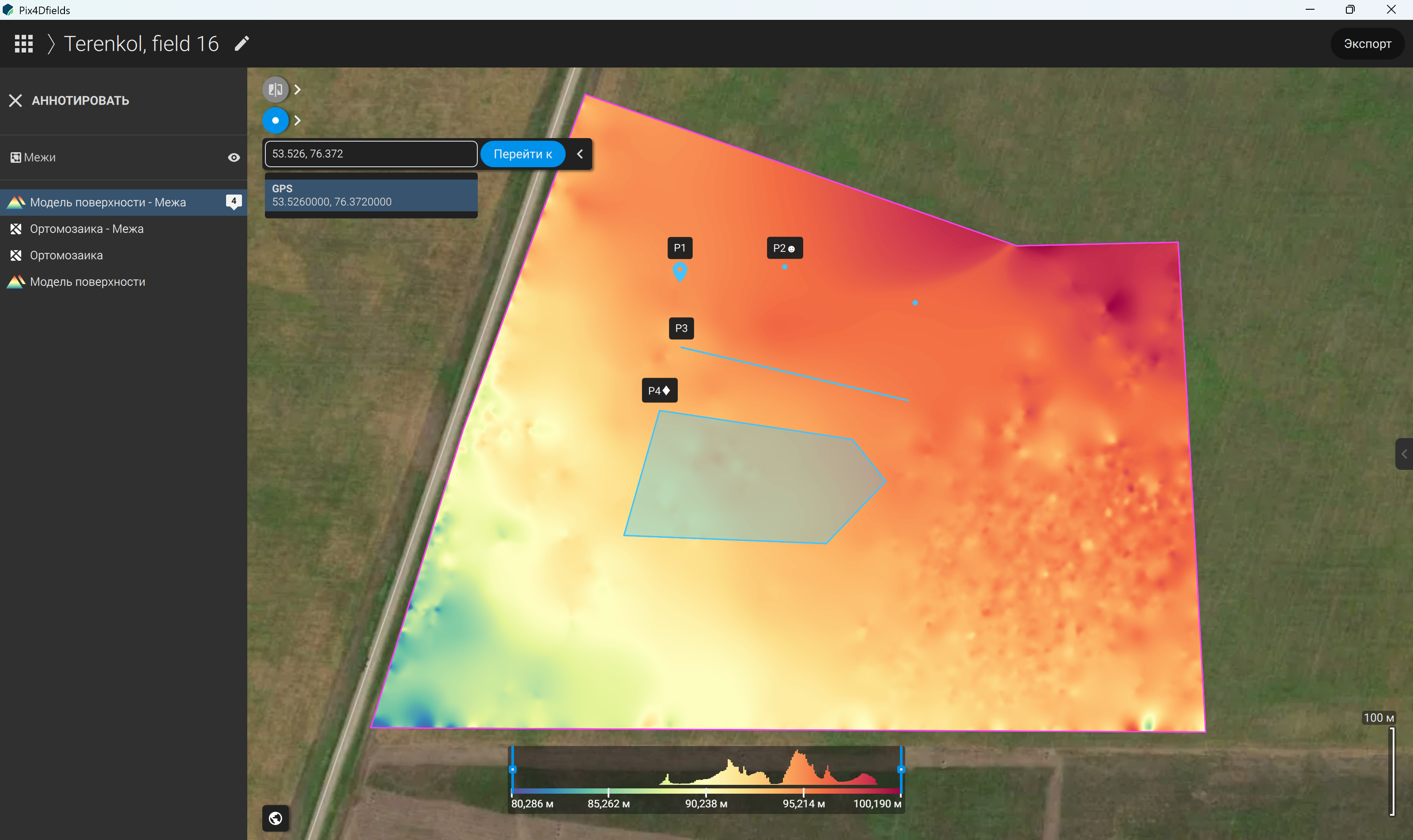
Figure 105 – Navigating to a location using a place name or GPS coordinates

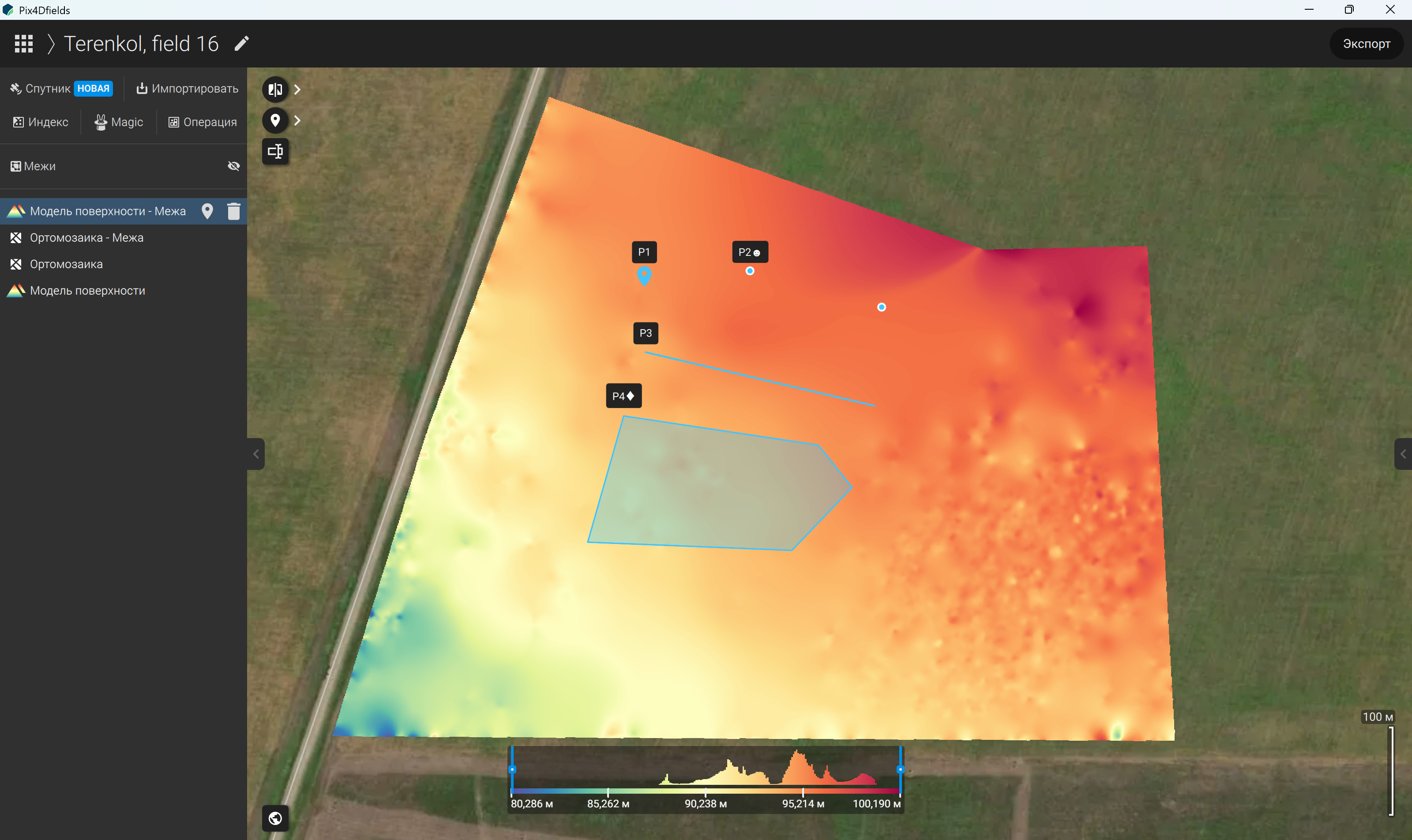
Figure 106 – Displaying the selected point on the map based on its GPS coordinates

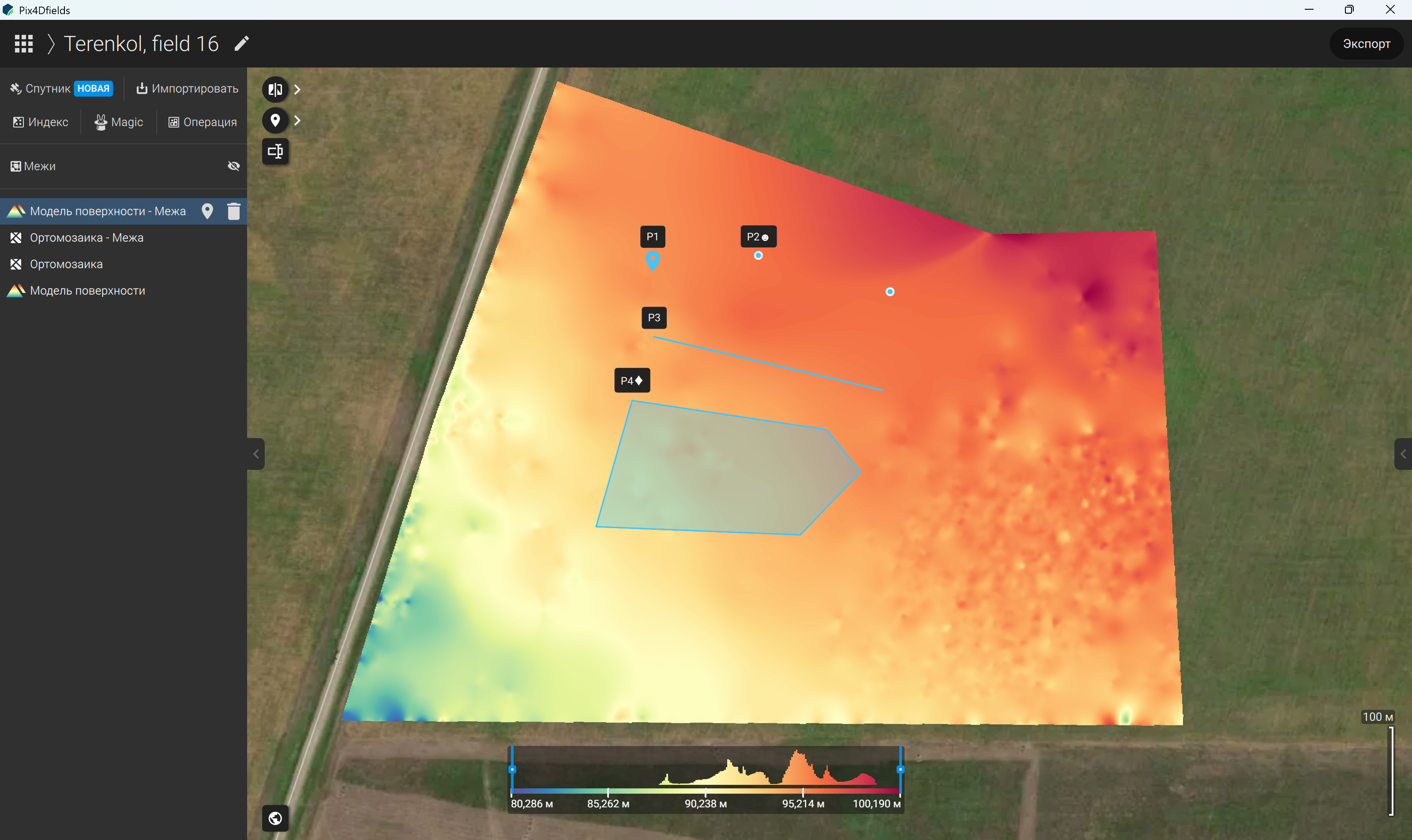
Figure 107 – Main data processing tools in the upper section of the left-hand panel

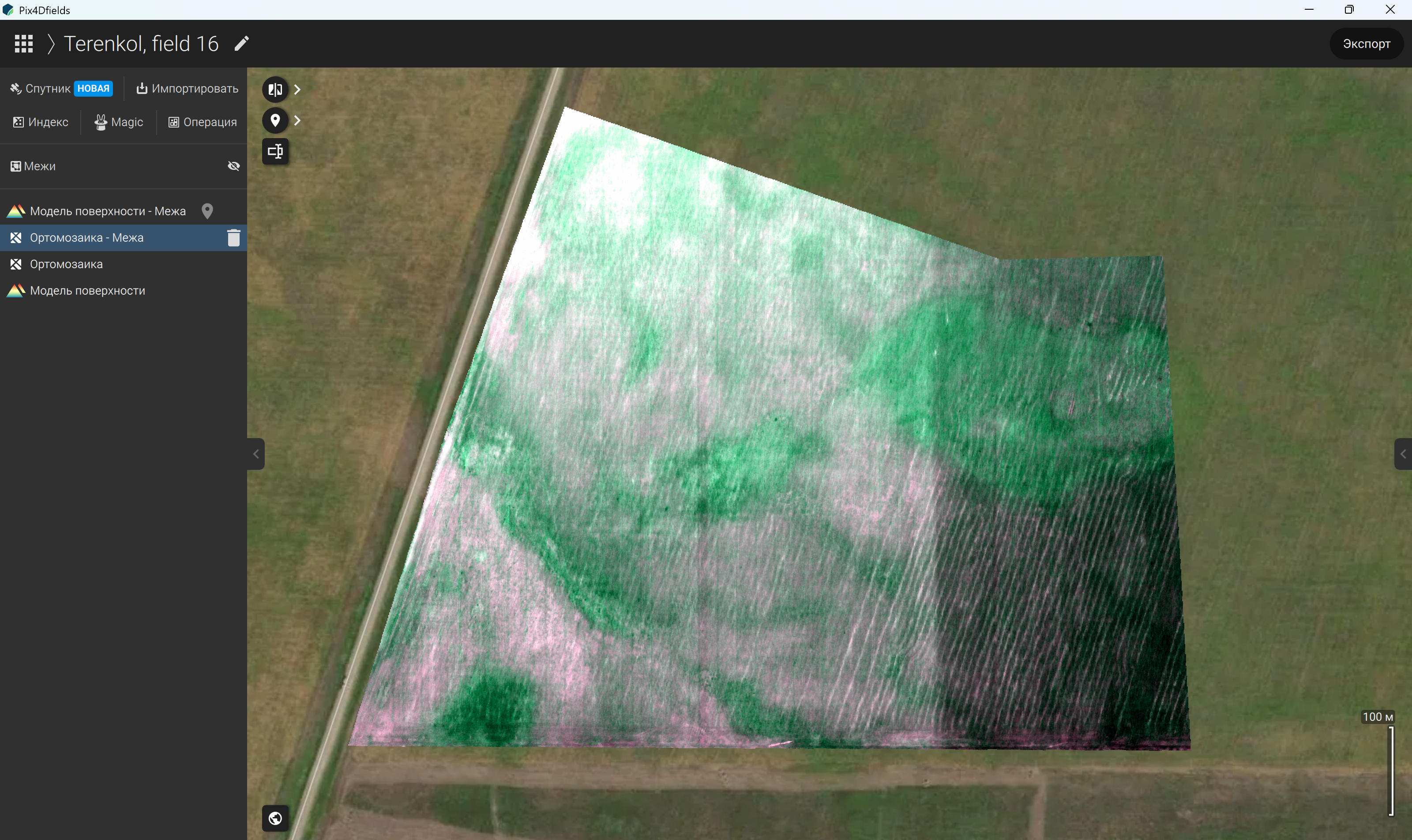
Figure 108 – Tools for importing supplementary satellite imagery and UAV images

Figure 109 – “Operation” tool for guided map processing

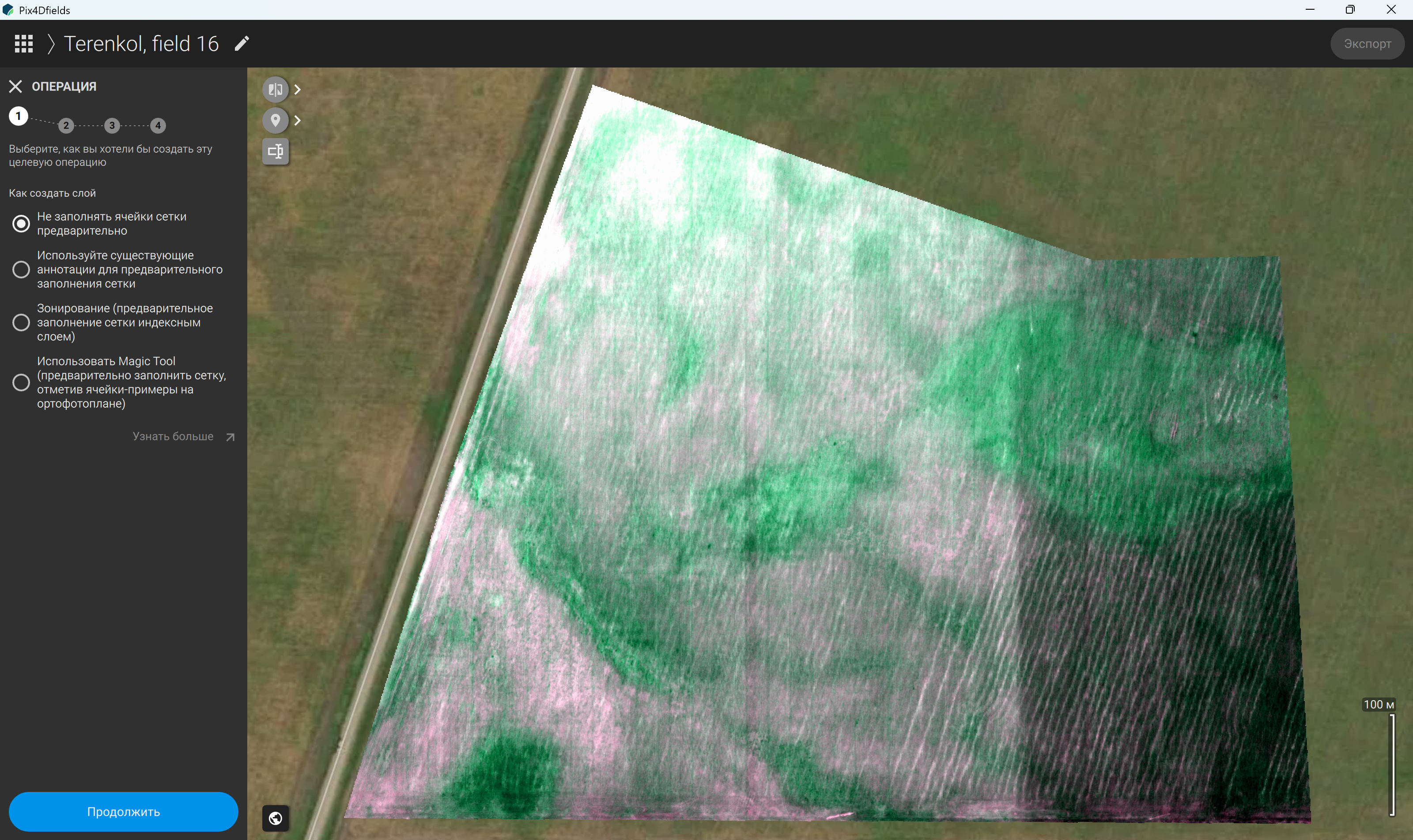
Figure 110 – Operation 1: Processing without pre-filling grid cells

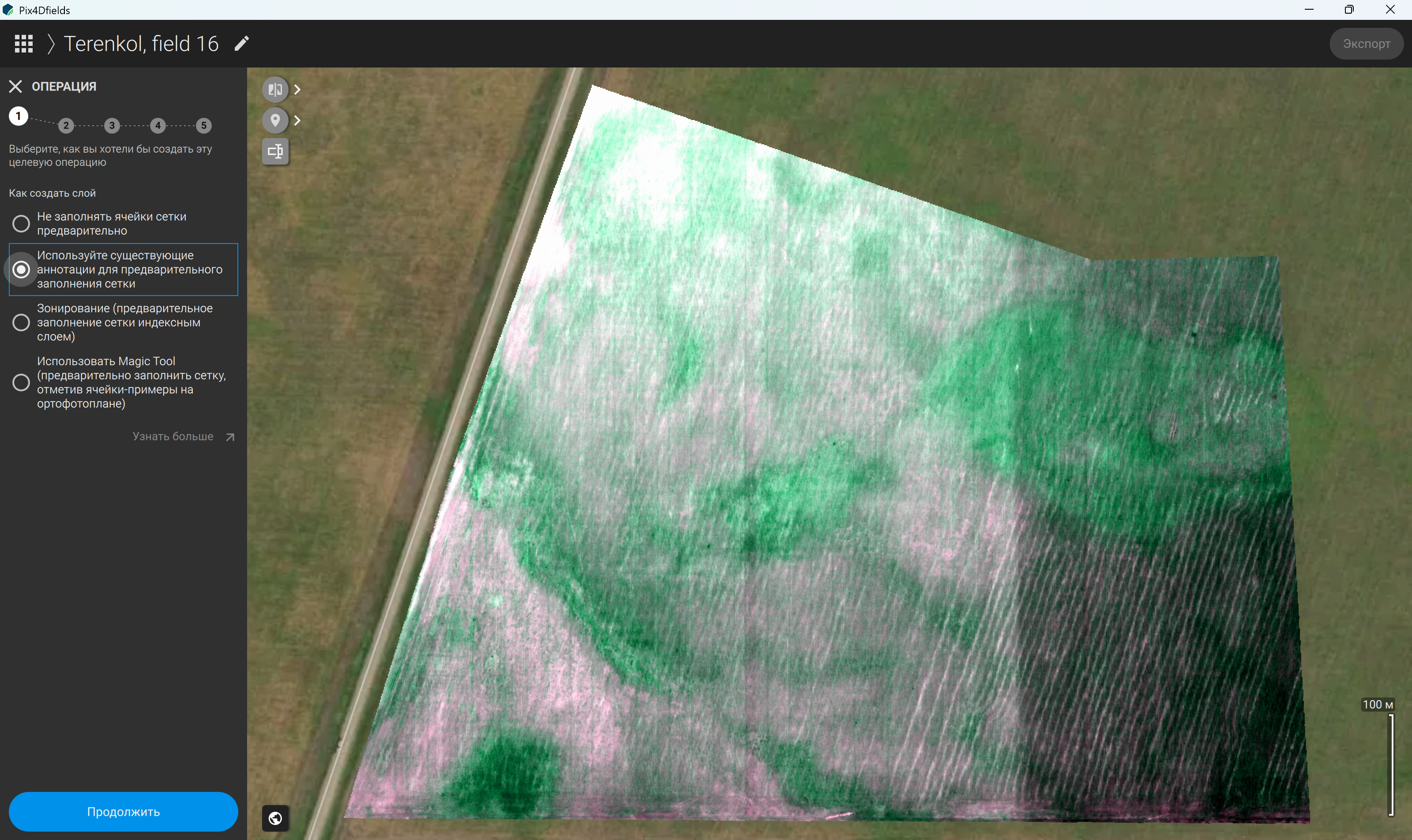
Figure 111 – Operation 2: Pre-filling the grid based on an annotation

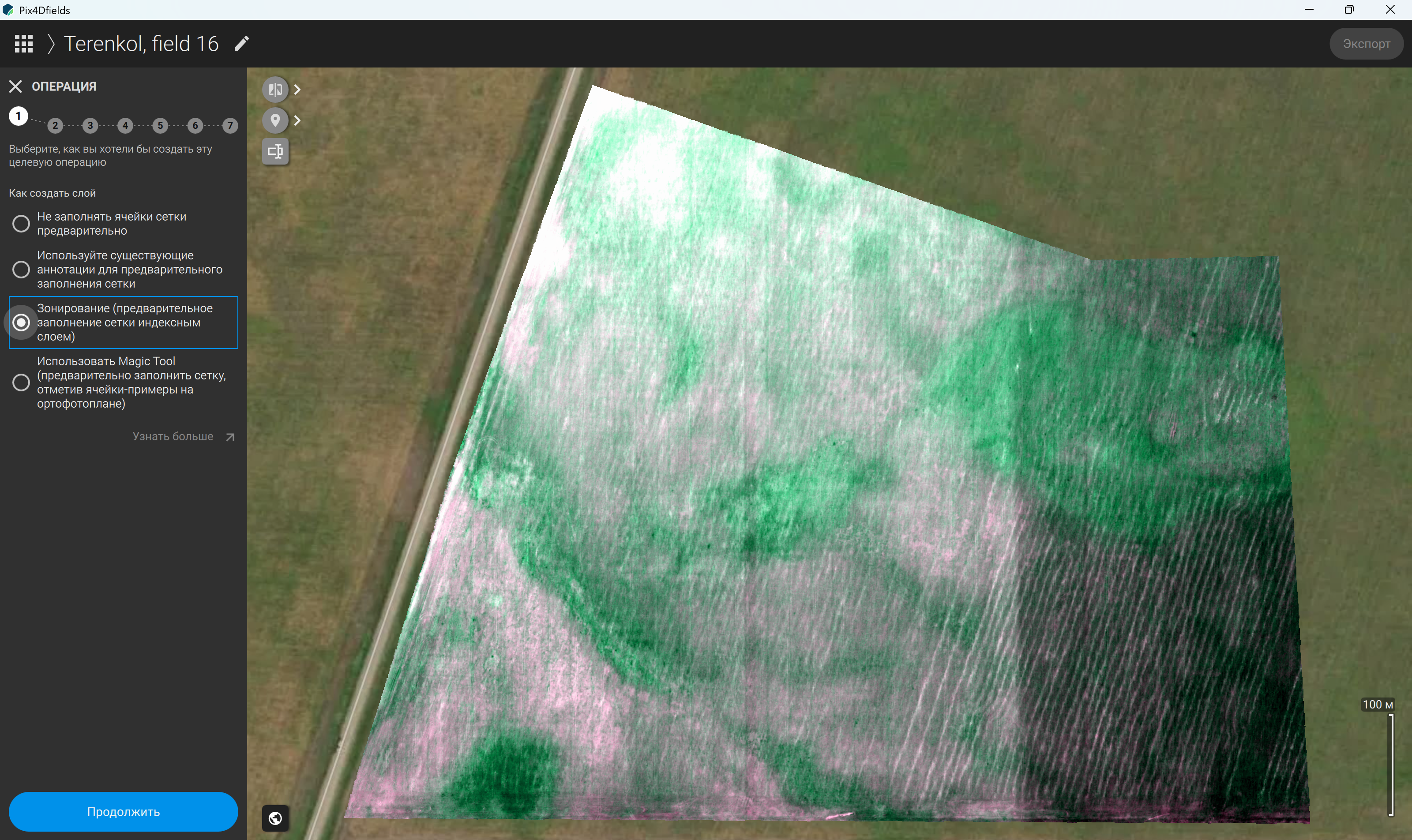
Figure 112 – Operation 3: Pre-filling the grid using an index layer for zoning

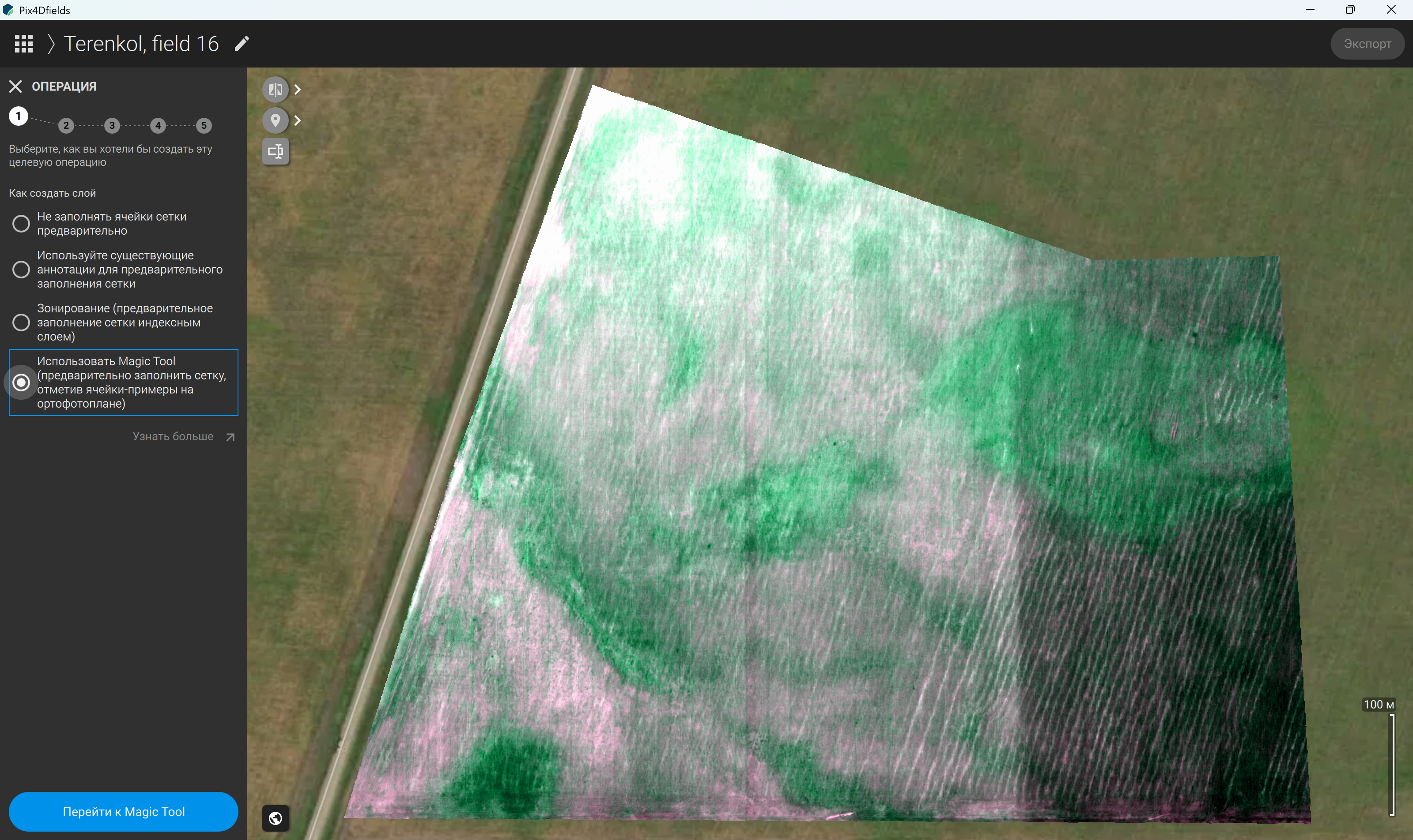
Figure 113 – Operation 4: Pre-filling the grid using orthomosaic reference cells with the Magic Tool

Figure 114 – “Magic Tool” for guided map processing

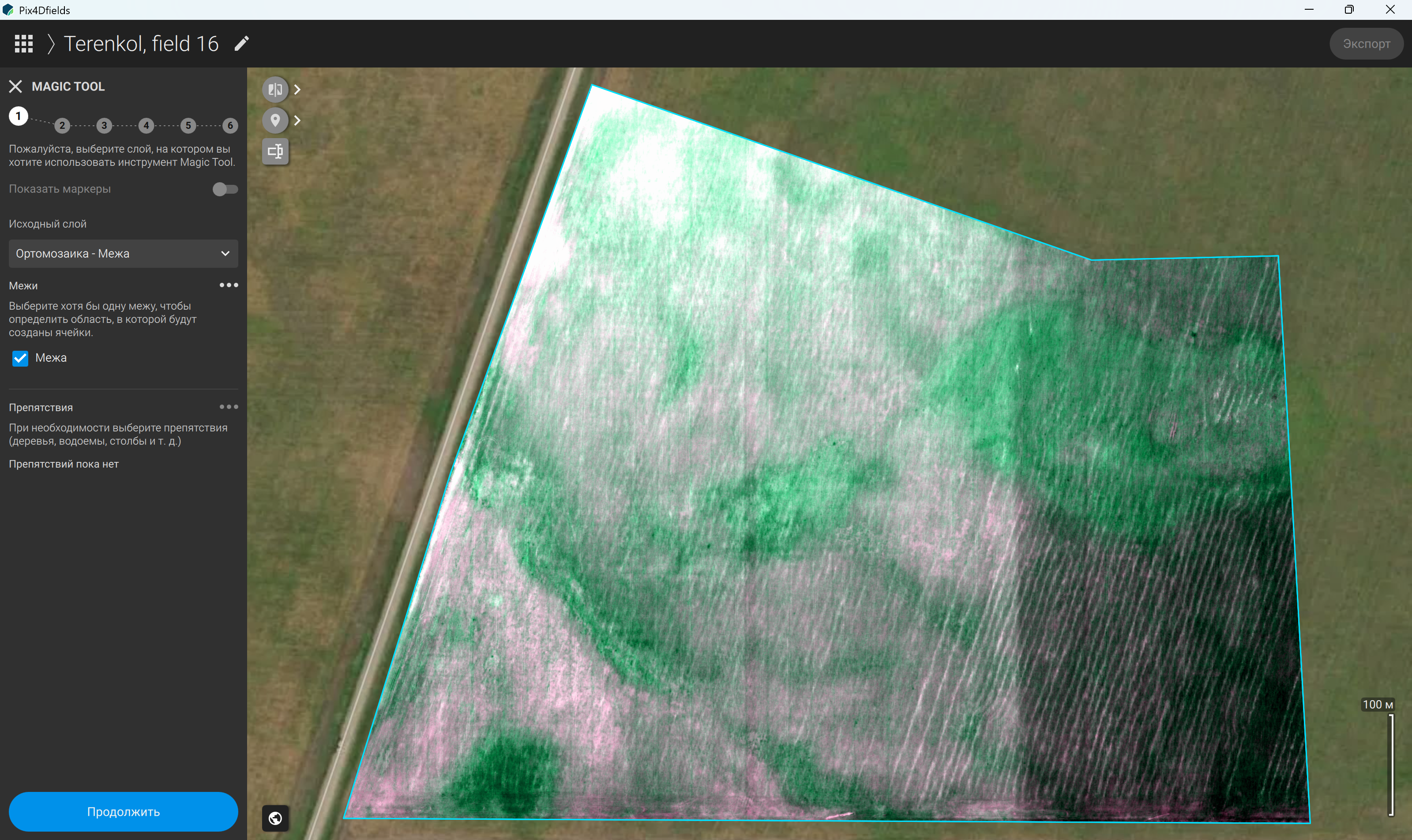
Figure 115 – Configuring the main “Magic Tool” parameters

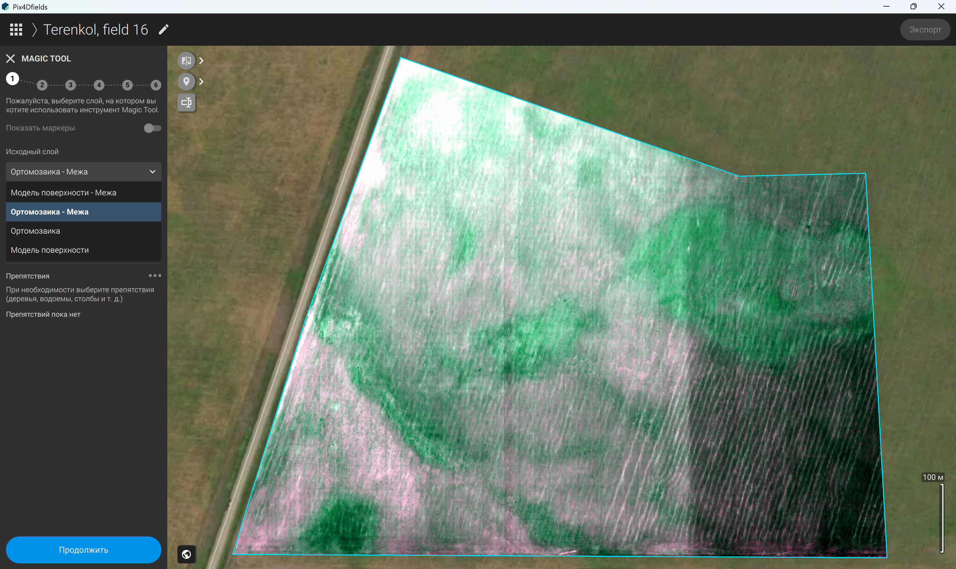
Figure 116 – Selecting the source layer and identifying obstacles for subsequent processing

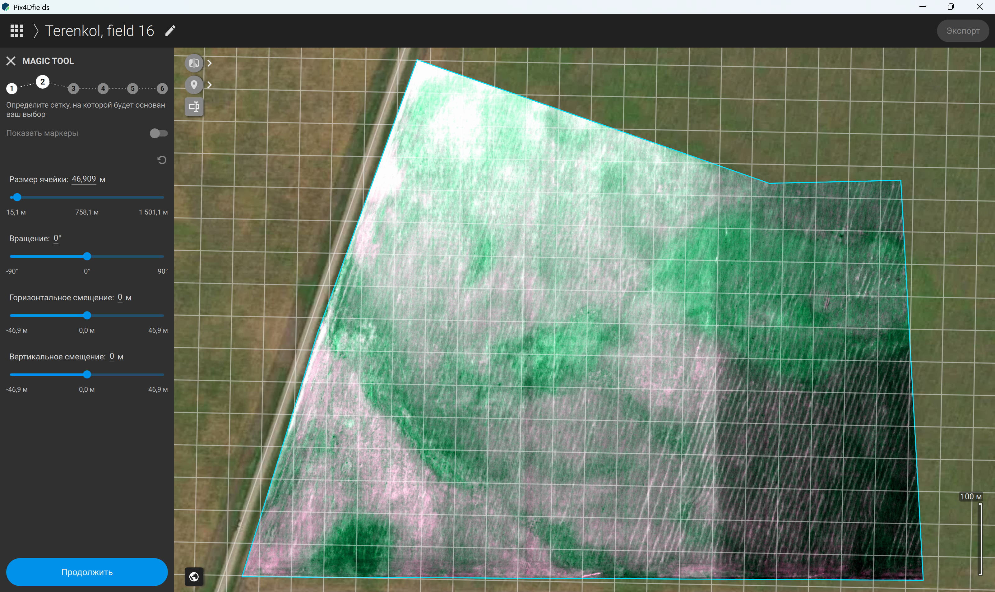
Figure 117 – Configuring grid parameters using the Magic Tool

Thus, the generation of a multispectral orthomosaic involves processing overlapping aerial images, combining them into a unified georeferenced representation of the surveyed area, and assessing the resulting data quality. The resulting orthomosaic provides the foundation for subsequent remote sensing analysis, including the calculation of spectral indices, the assessment of crop health, the delineation of vegetation variability zones, and the preparation of prescription maps for precision agriculture.