5 Calculation and analysis of vegetation indices for assessing the condition of agricultural crops

The calculation and analysis of vegetation indices are essential steps in assessing the condition of agricultural crops using remote sensing data.

Modern agriculture increasingly incorporates Earth observation technologies and unmanned aerial vehicles into routine field monitoring. These technologies enable the rapid acquisition of crop condition data, the identification of potentially problematic areas, and the timely implementation of appropriate crop management measures. Vegetation indices are among the most widely used tools for analysing such data. A vegetation index is a mathematical measure derived from the reflectance values of vegetation in one or more spectral bands. Healthy vegetation typically absorbs a substantial proportion of visible red radiation for photosynthesis while reflecting strongly in the near-infrared (NIR) region. These spectral characteristics can be used to assess vegetation vigour, identify spatial variations in crop development, and detect potential stress conditions.

Once image processing and orthomosaic generation have been completed, vegetation indices can be calculated. To do this, the user selects the “Index” tool at the top of the left-hand panel (Figure 118), which opens the “Index Generator” window (Figure 119). The previously generated orthomosaic is selected as the input layer, after which the available vegetation indices are displayed. The range of available indices depends on the spectral bands provided by the input imagery and the capabilities of the software. For multispectral imagery, commonly available indices include NDVI, NDRE, GNDVI, MCARI, and LCI. For imagery acquired using an RGB camera, indices that rely exclusively on visible spectral bands, such as VARI and SIPI2, may be available. Other indices require additional spectral information and therefore cannot be calculated from RGB imagery alone. To generate a vegetation index map, the required index is selected and the “Generate” button is clicked (Figure 119). The software then calculates the index and creates a corresponding thematic layer, such as an NDVI map (Figure 120). After the NDVI layer has been generated, its visualisation settings can be accessed through the “View” section (Figure 121), while the “Info” section provides information about the layer (Figure 122). The same procedure can be used to generate maps of other supported vegetation indices (Figure 123), producing the corresponding thematic layers (Figures 124-128).

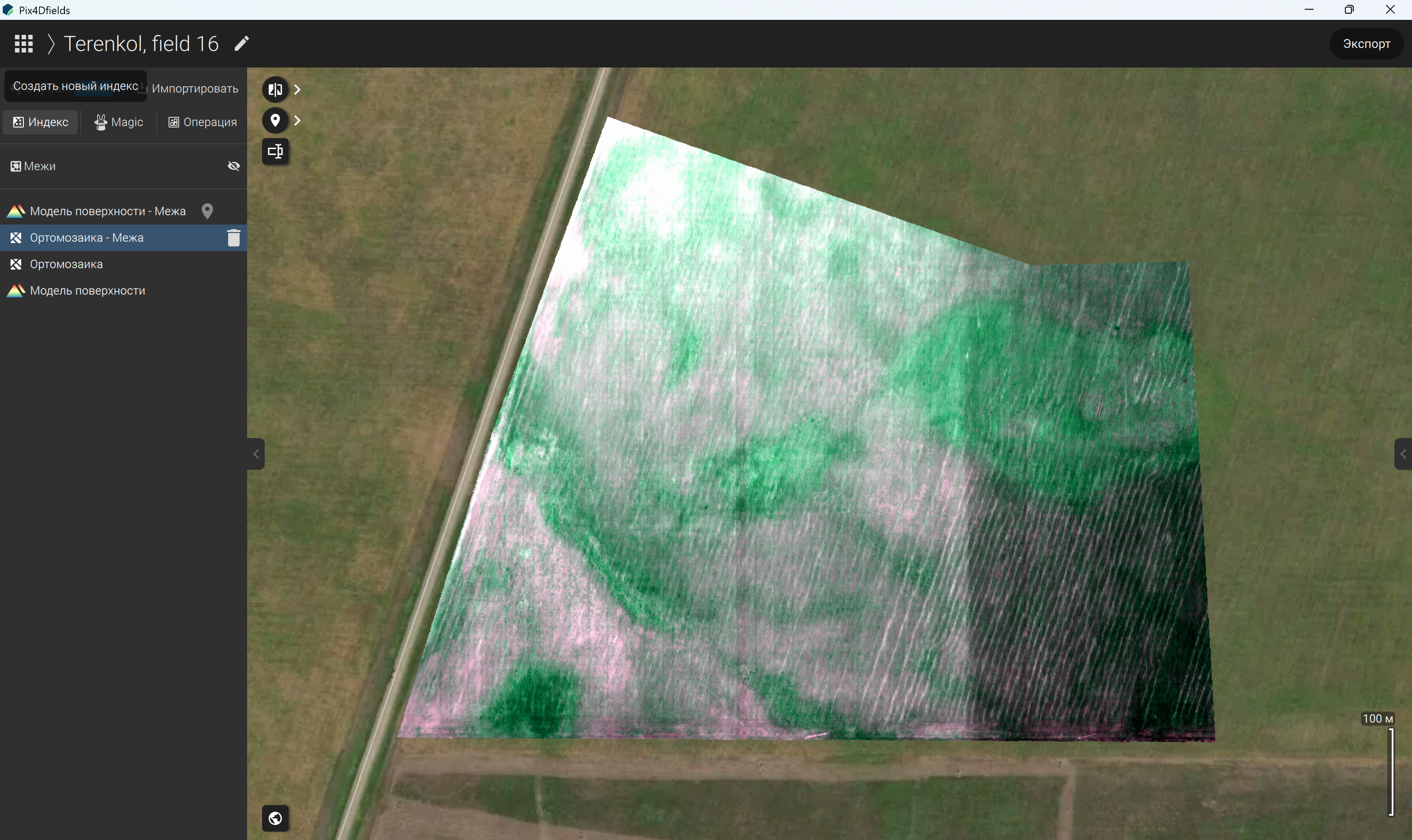
Figure 118 – “Index” tool

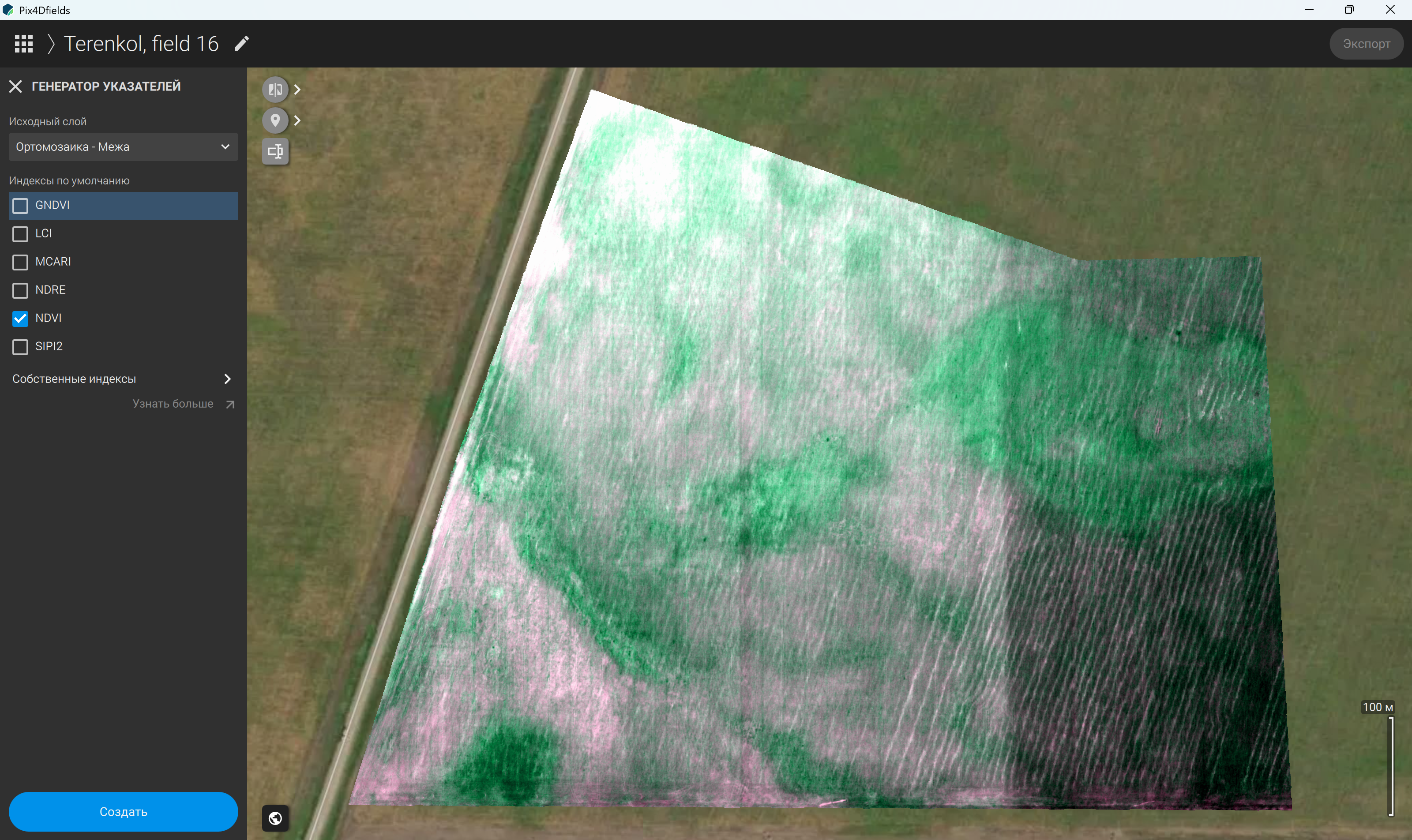
Figure 119 – Selecting the default NDVI index in the “Index Generator” window

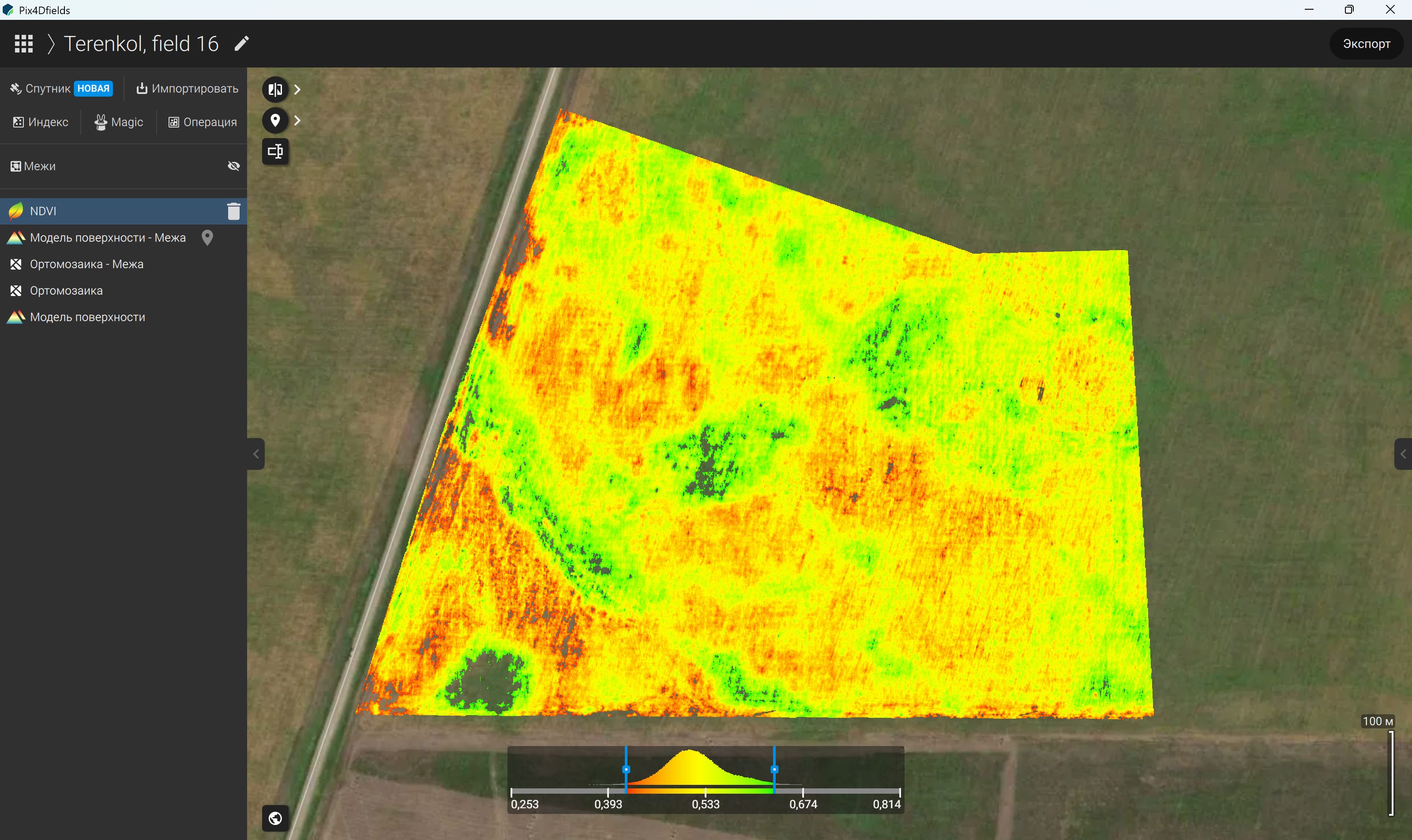
Figure 120 – Generated NDVI map

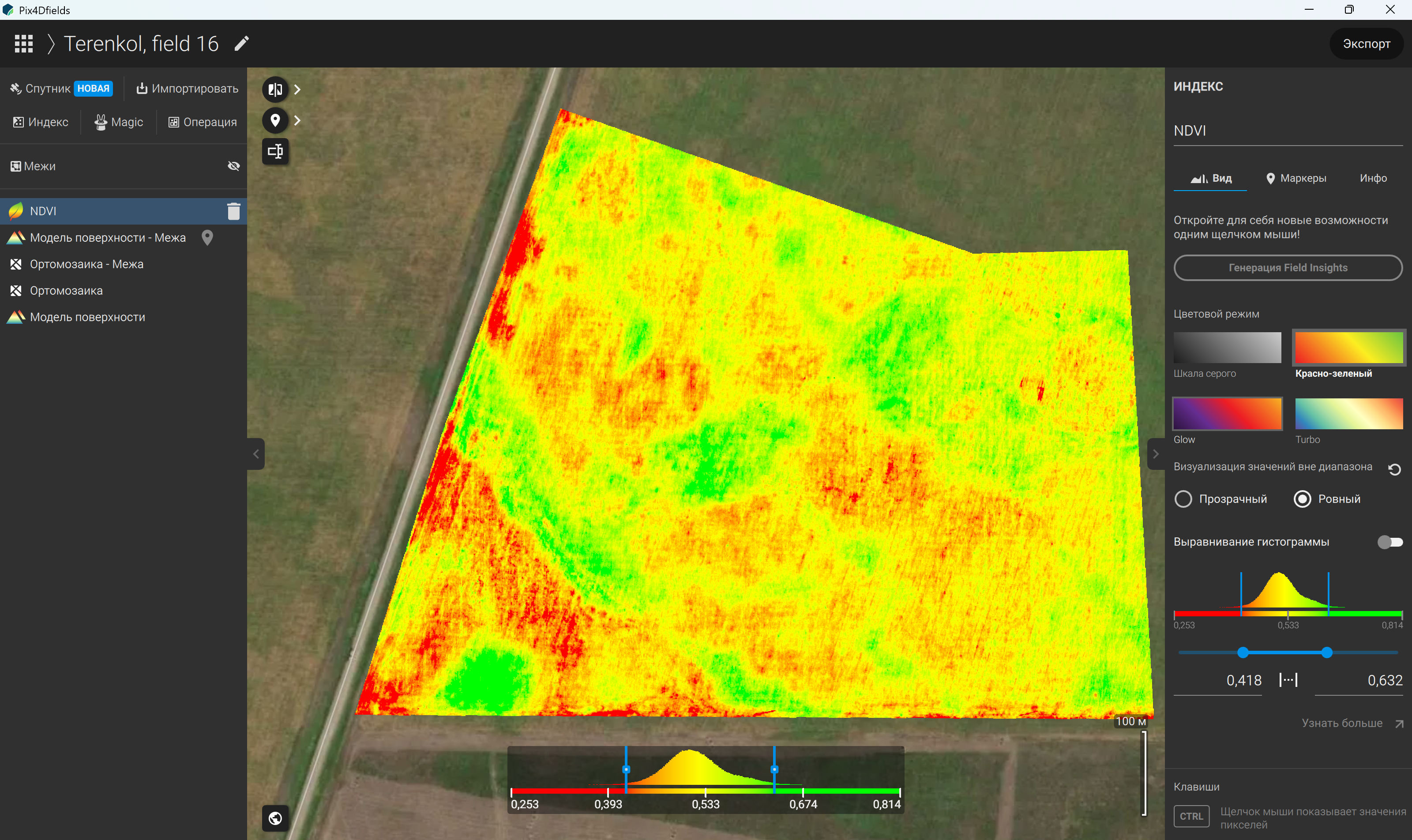
Figure 121 – “View” section of the NDVI layer, including colour display and equalisation settings

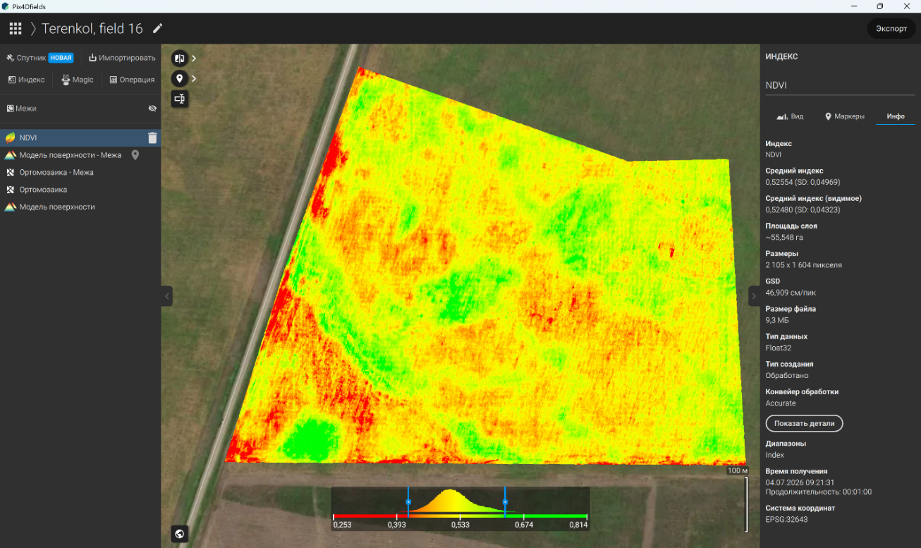
Figure 122 – Information displayed in the “Info” section of the NDVI layer

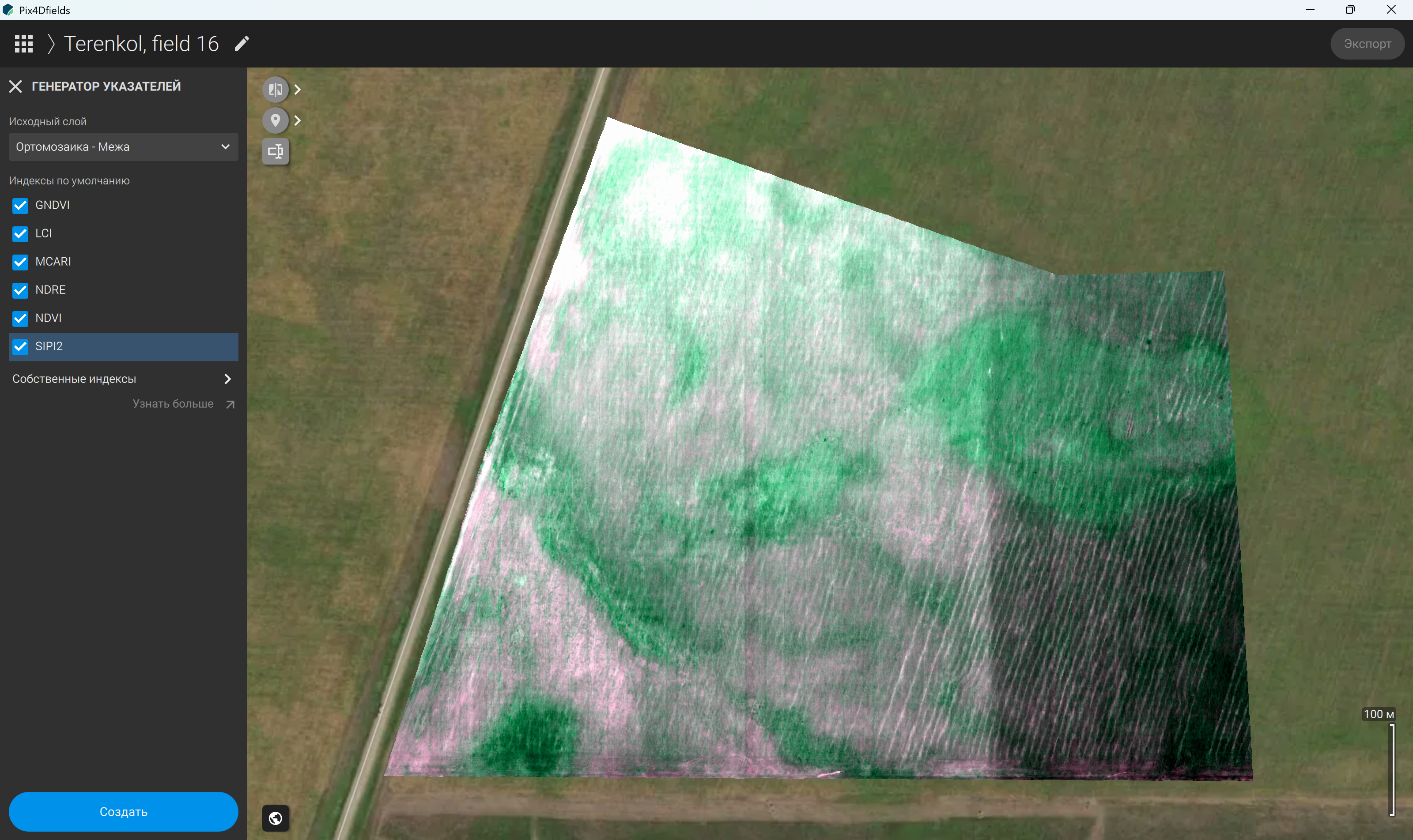
Figure 123 – Selecting the available vegetation indices in the “Index Generator” window

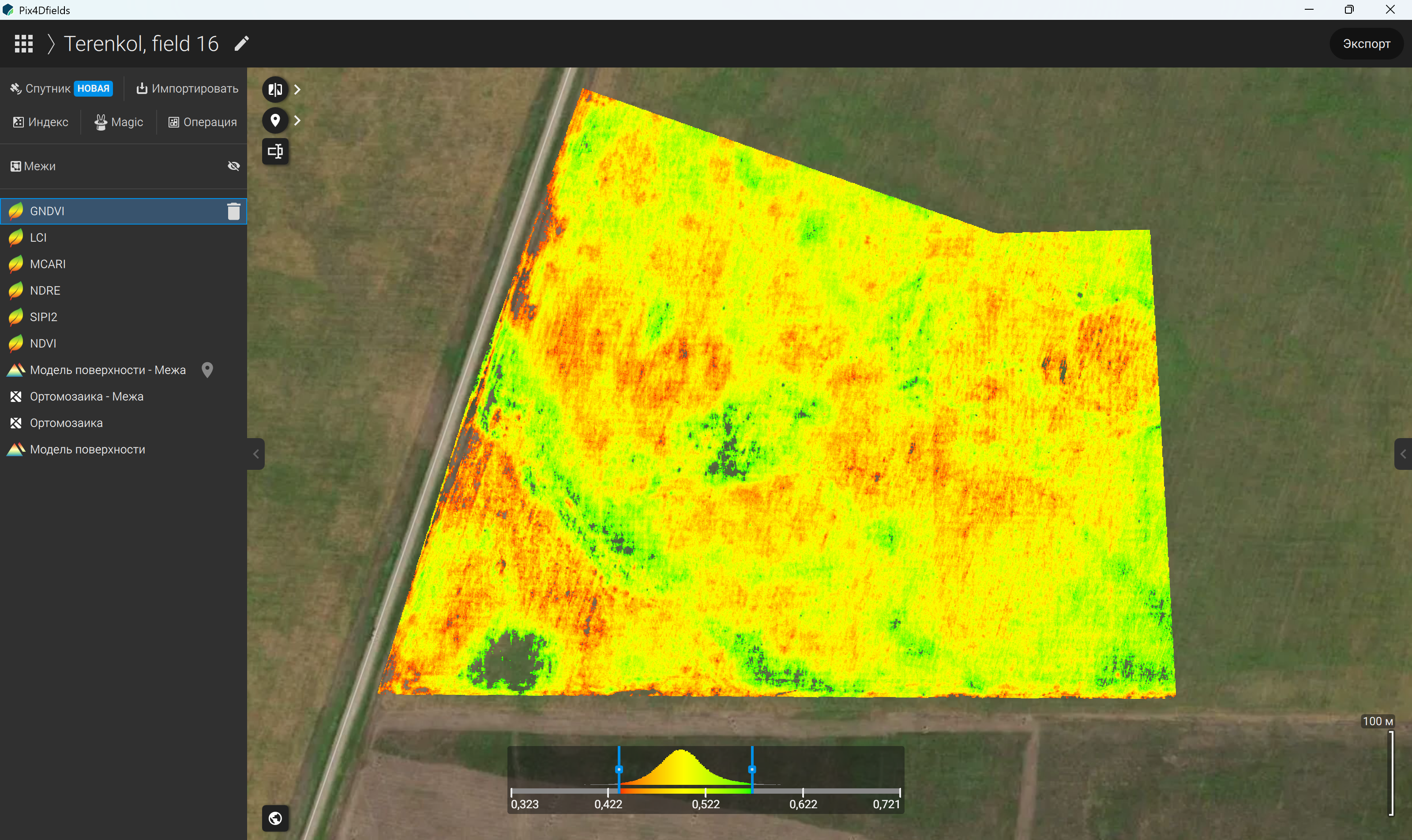
Figure 124 – GNDVI index map

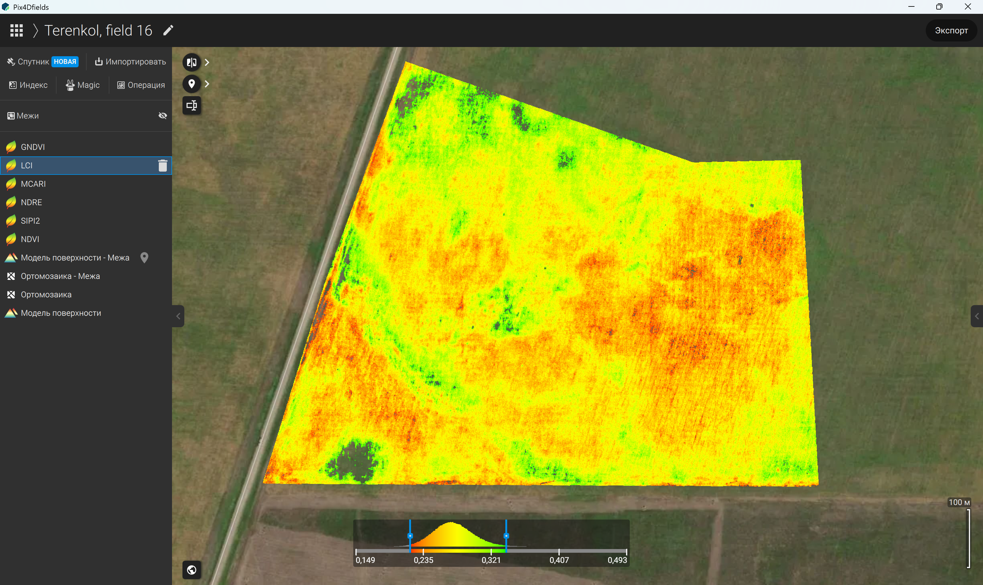
Figure 125 – LCI index map

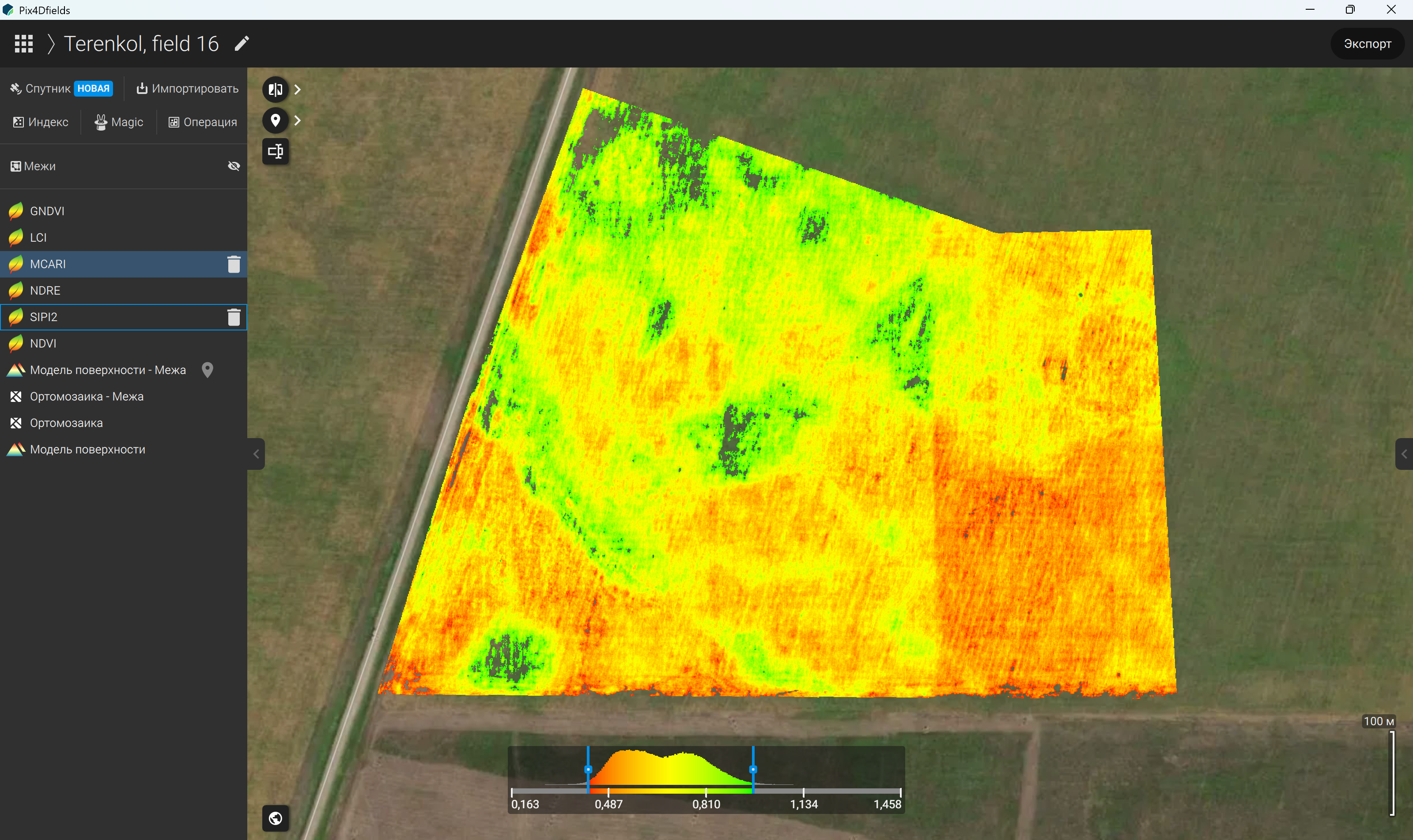
Figure 126 – MCARI index map

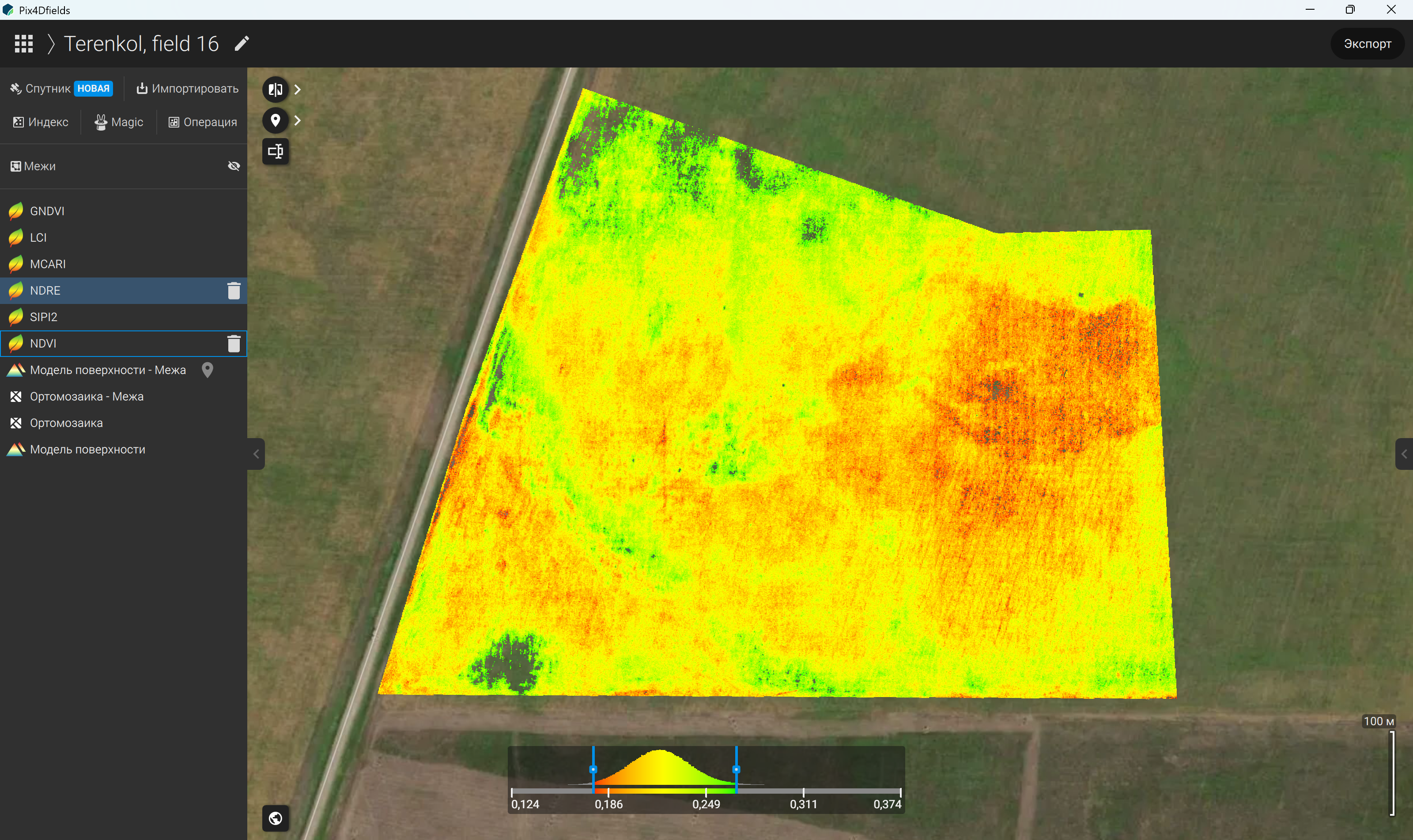
Figure 127 – NDRE index map

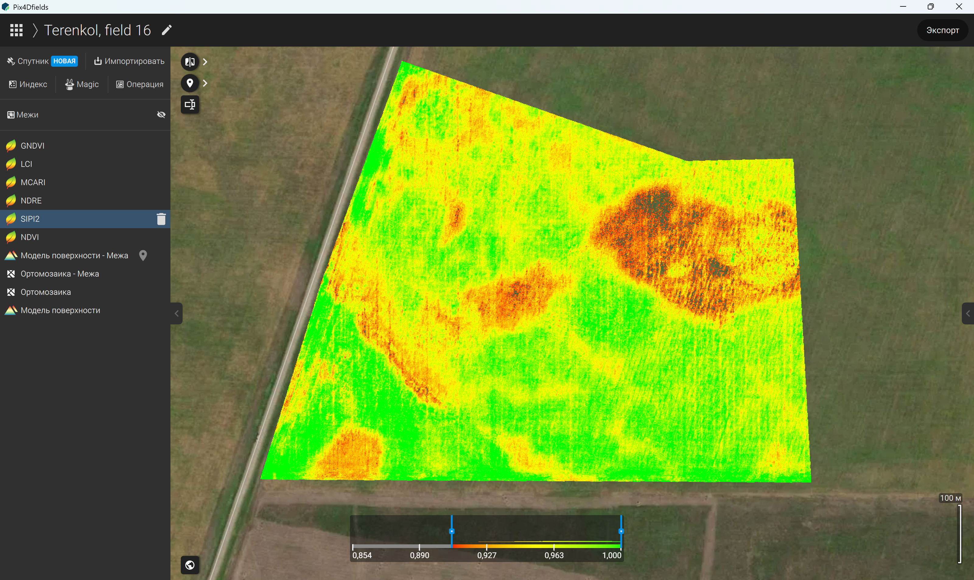
Figure 128 – SIPI2 index map

Pix4Dfields also provides functionality for calculating custom vegetation indices (Figure 129) using the built-in index calculator (Figure 130). First, the input layer, typically the orthomosaic, is selected. The required index can then be selected or defined in the “Index” field, where the corresponding calculation formula may be displayed automatically for supported indices. Alternatively, the user can construct a custom formula using the available spectral bands and mathematical operations (Figure 131). Before generating the final map, the “Preview” function can be used to inspect the calculated results (Figure 132). Once the formula and input data have been checked, the user clicks “Apply”, and the software generates the corresponding thematic layer (Figure 133).

The resulting map represents the spatial distribution of the selected vegetation index. Its colours correspond to different index values and help reveal variations in vegetation characteristics across the surveyed area. For example, low NDVI values may indicate sparse vegetation, exposed soil, reduced canopy development, or potential plant stress, whereas higher values generally indicate greater green vegetation cover and vigour. However, the interpretation depends on the index used, the growth stage of the crop, soil background effects, and the conditions under which the imagery was acquired. Consequently, index values should not be interpreted as definitive evidence of a specific stress factor without additional information. The map's visualisation can be customised through the “View” section in the right-hand panel (Figure 134). Available display options may include Greyscale (Figure 135), Glow (Figure 136), and Turbo (Figure 137). Users can also adjust the displayed value range and layer transparency to facilitate visual interpretation and comparison of spatial patterns.

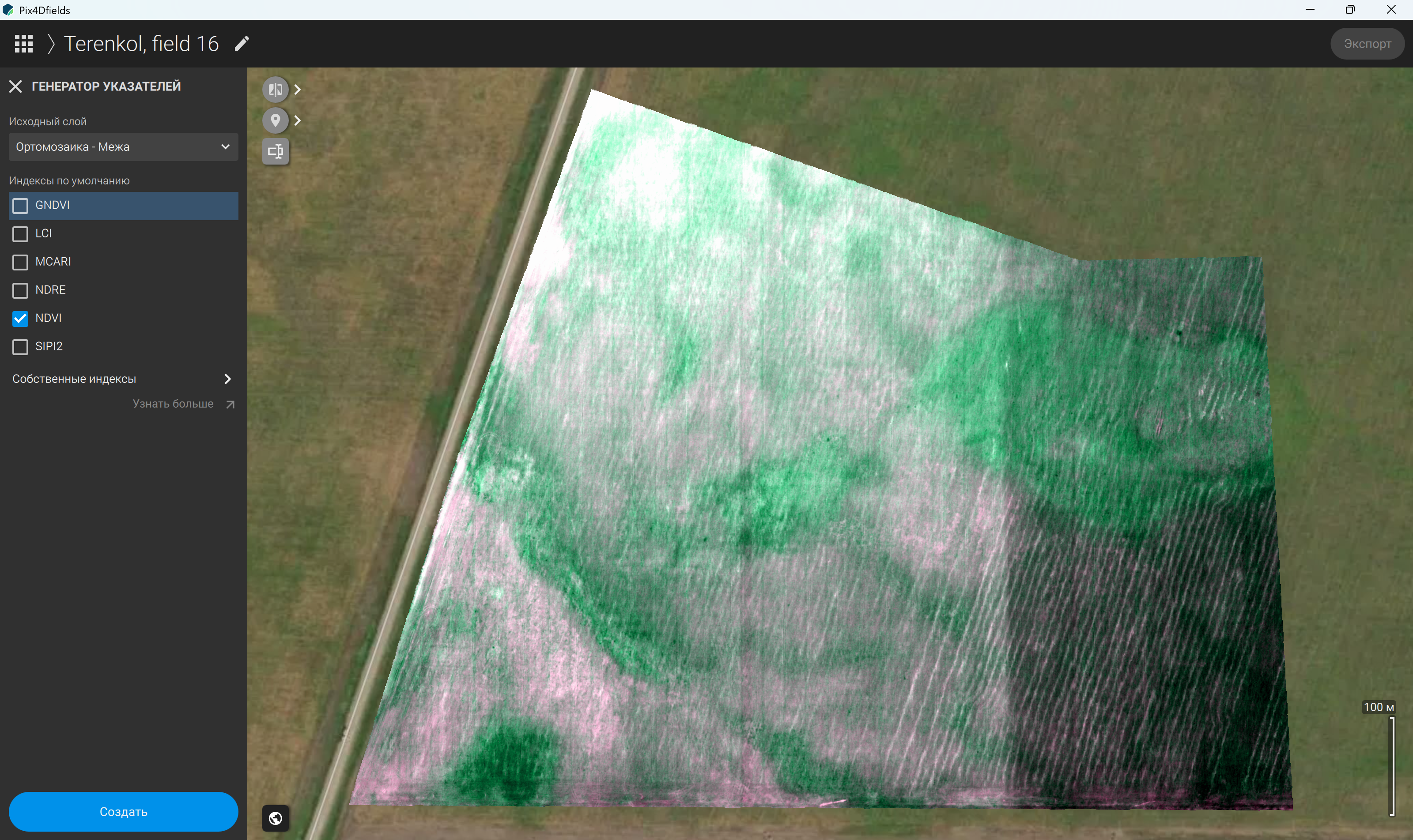
Figure 129 – Selecting the custom index creation function

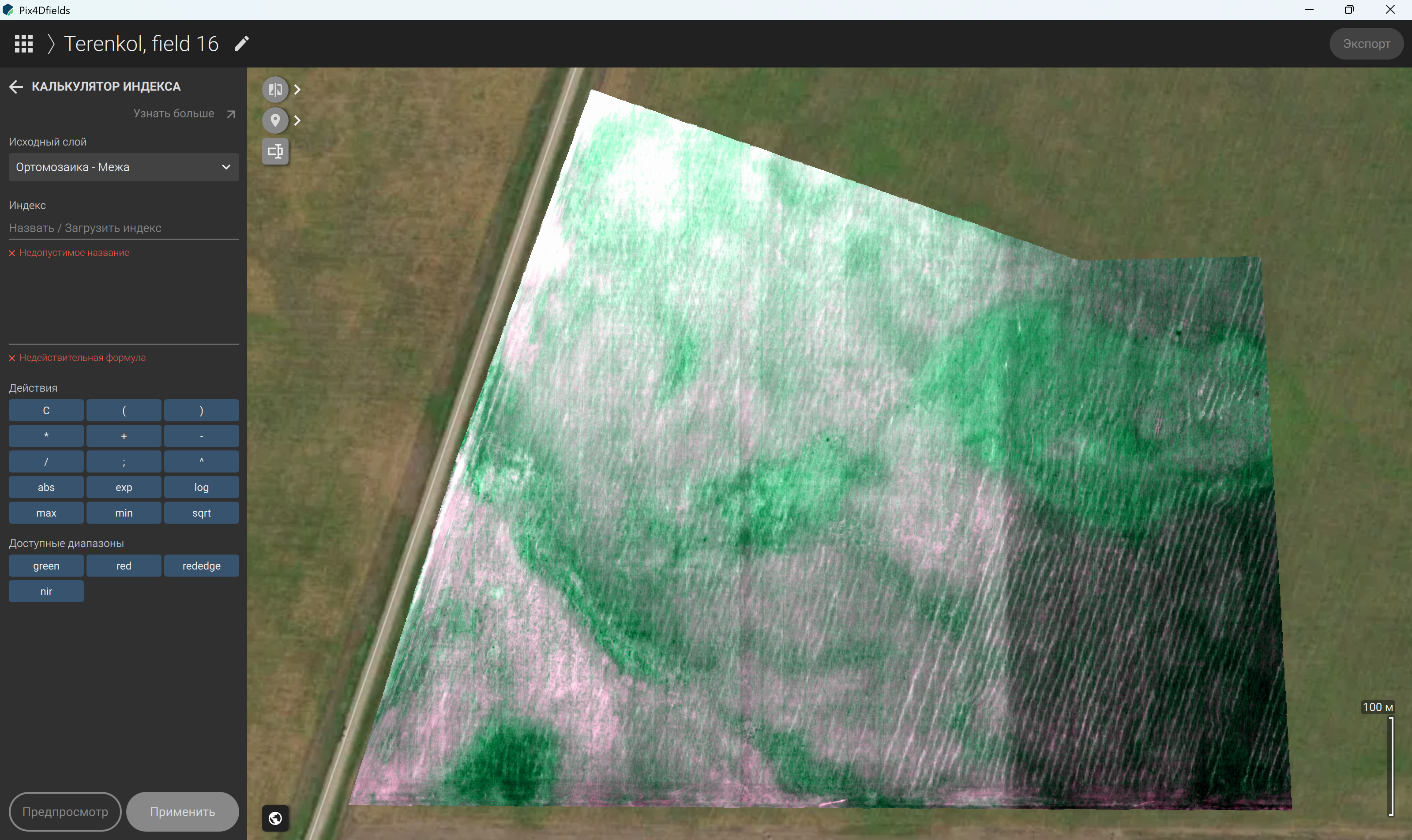
Figure 130 – Opening the index calculator

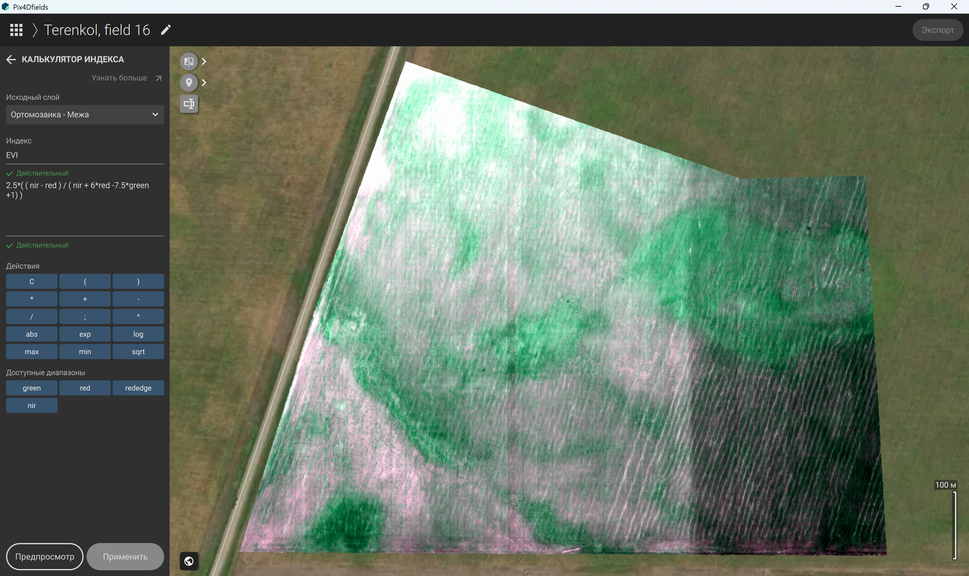
Figure 131 – Selecting the input layer and defining the index formula in the calculator

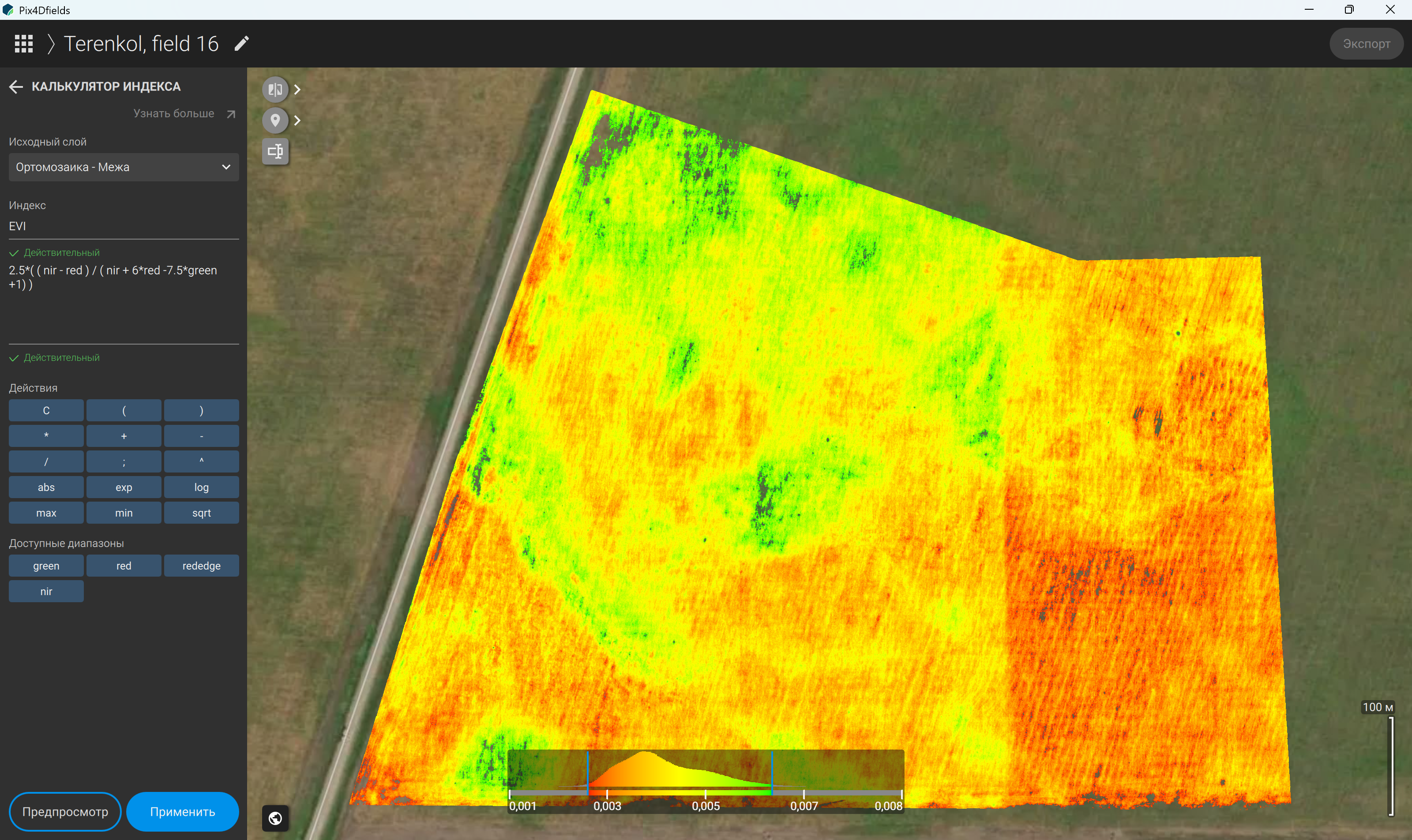
Figure 132 – Previewing the calculated vegetation index map

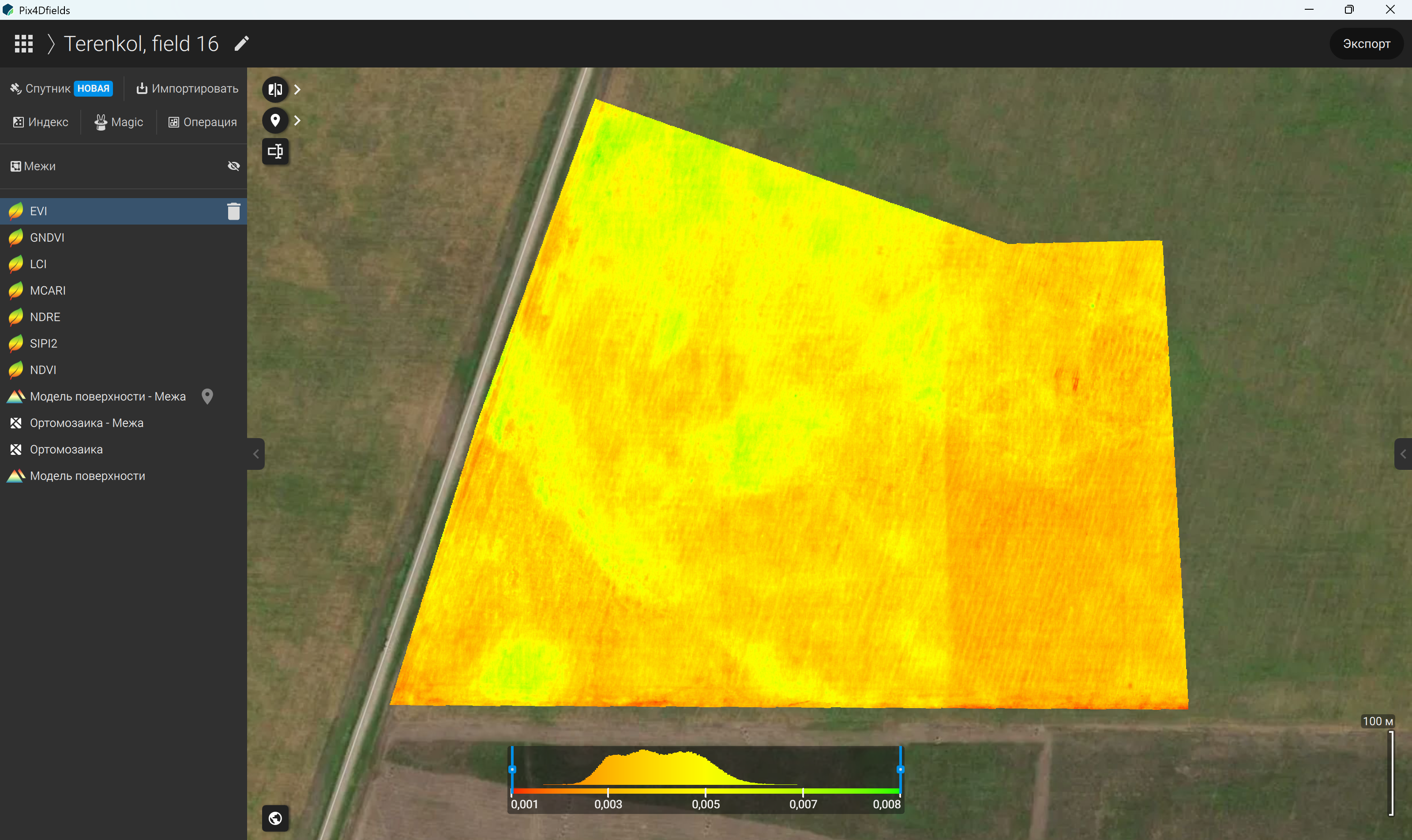
Figure 133 – Generated custom vegetation index map

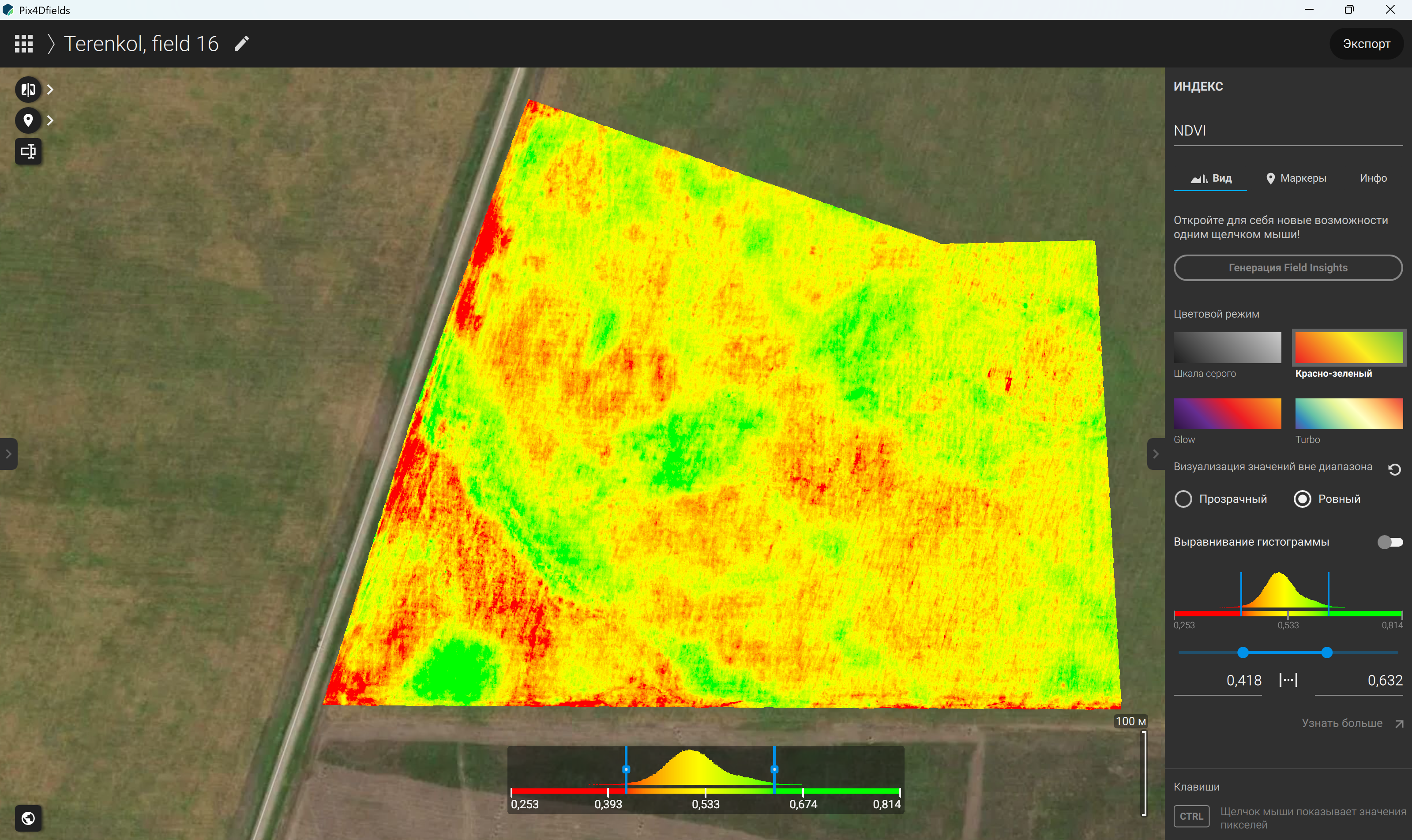
Figure 134 – “View” section of the NDVI layer

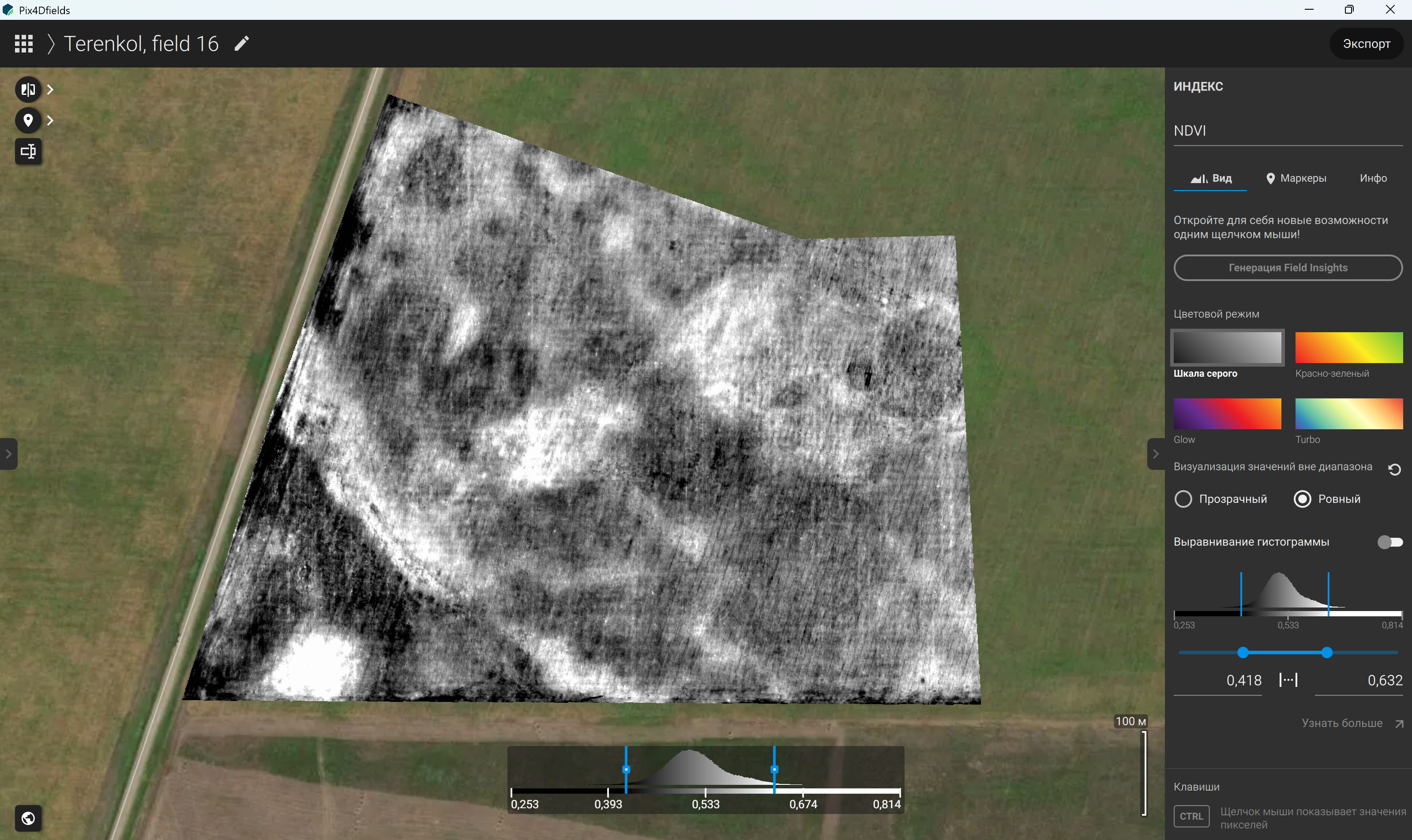
Figure 135 – Displaying the NDVI map using the Greyscale colour scheme

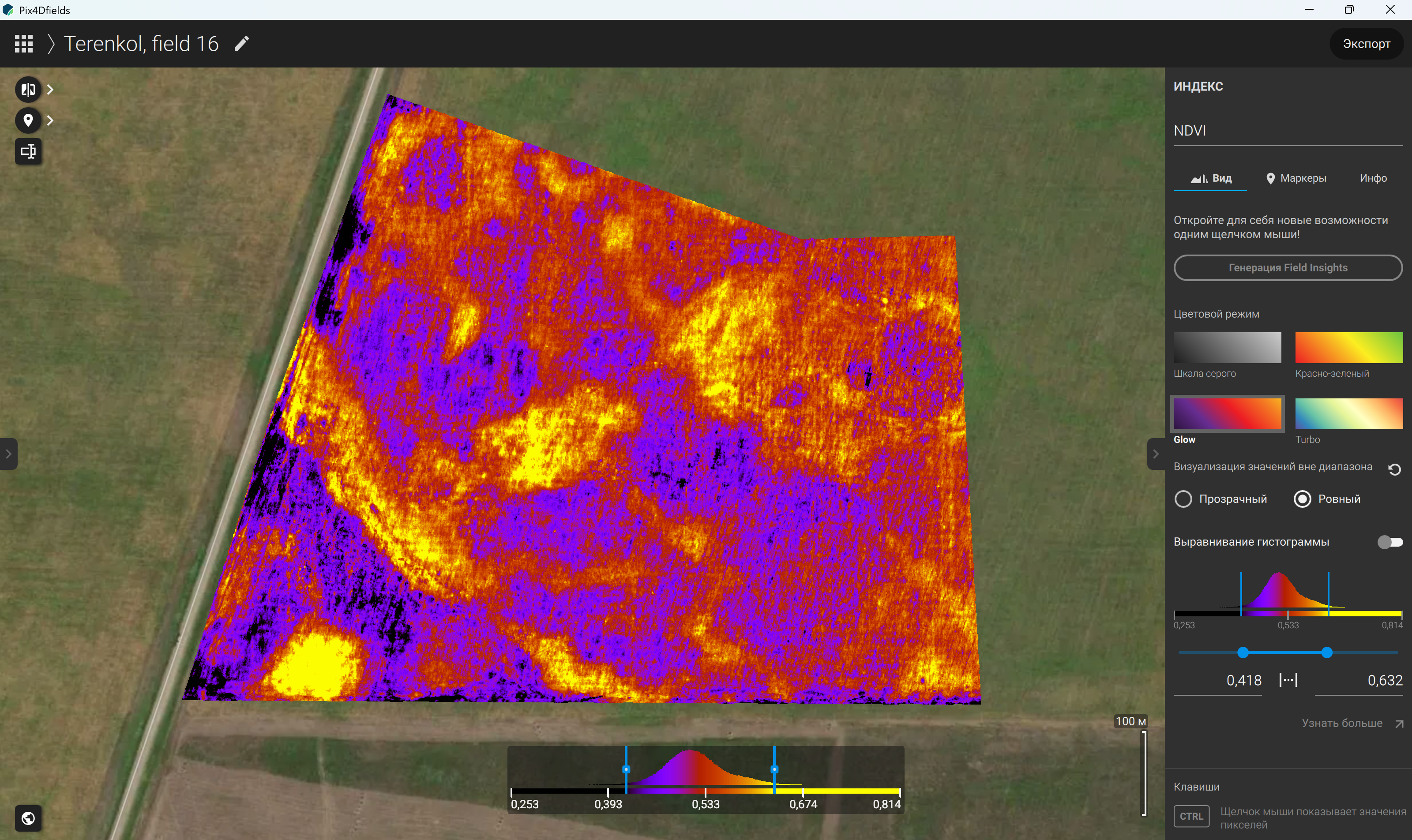
Figure 136 – Displaying the NDVI map using the Glow colour scheme

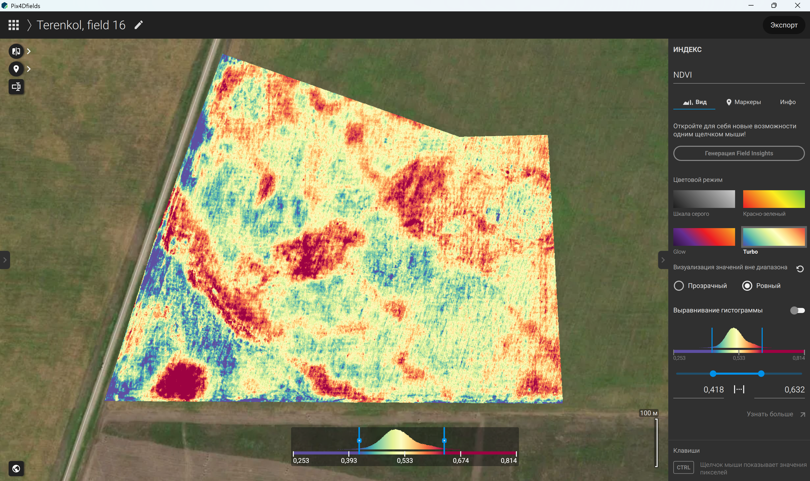
Figure 137 – Displaying the NDVI map using the Turbo colour scheme

Once the vegetation index maps have been generated and reviewed, the resulting data can be exported for further analysis, documentation, and reporting. To begin, the user selects the “Export” command in the top menu bar (Figure 138), which opens the Export Wizard (Figure 139). The Export Wizard provides options for sharing processed data and generated maps (Figure 140), selecting the layers to be exported (Figure 141), exporting layer statistics (Figure 142), and selecting field boundaries (Figure 143) and annotations or markers (Figure 144). It also allows users to configure image export settings (Figure 145) and specify the appearance of exported markers (Figure 146). In addition, a PDF report can be generated by selecting the required report content (Figure 147) and the layers to be included (Figure 148). After selecting the required layers, the user clicks “Continue” and configures the export parameters. Depending on the selected output format, these settings may include the output data type, image resolution or scale, and the use of image pyramids. The destination folder for the exported files is then specified. To generate a PDF report, the corresponding report options are selected in the Export Wizard. The user chooses the layers to include, enters a report title and project description, and selects a standard or custom report template, where available. Additional display settings can then be configured, including marker colours (Figure 147) and the visibility of the basemap (Figure 148). After all parameters have been reviewed, the user clicks “Export” to generate and save the report. The resulting files can subsequently be used for documenting field conditions, comparing vegetation index maps, identifying spatial variations in crop development, and supporting agricultural management decisions.

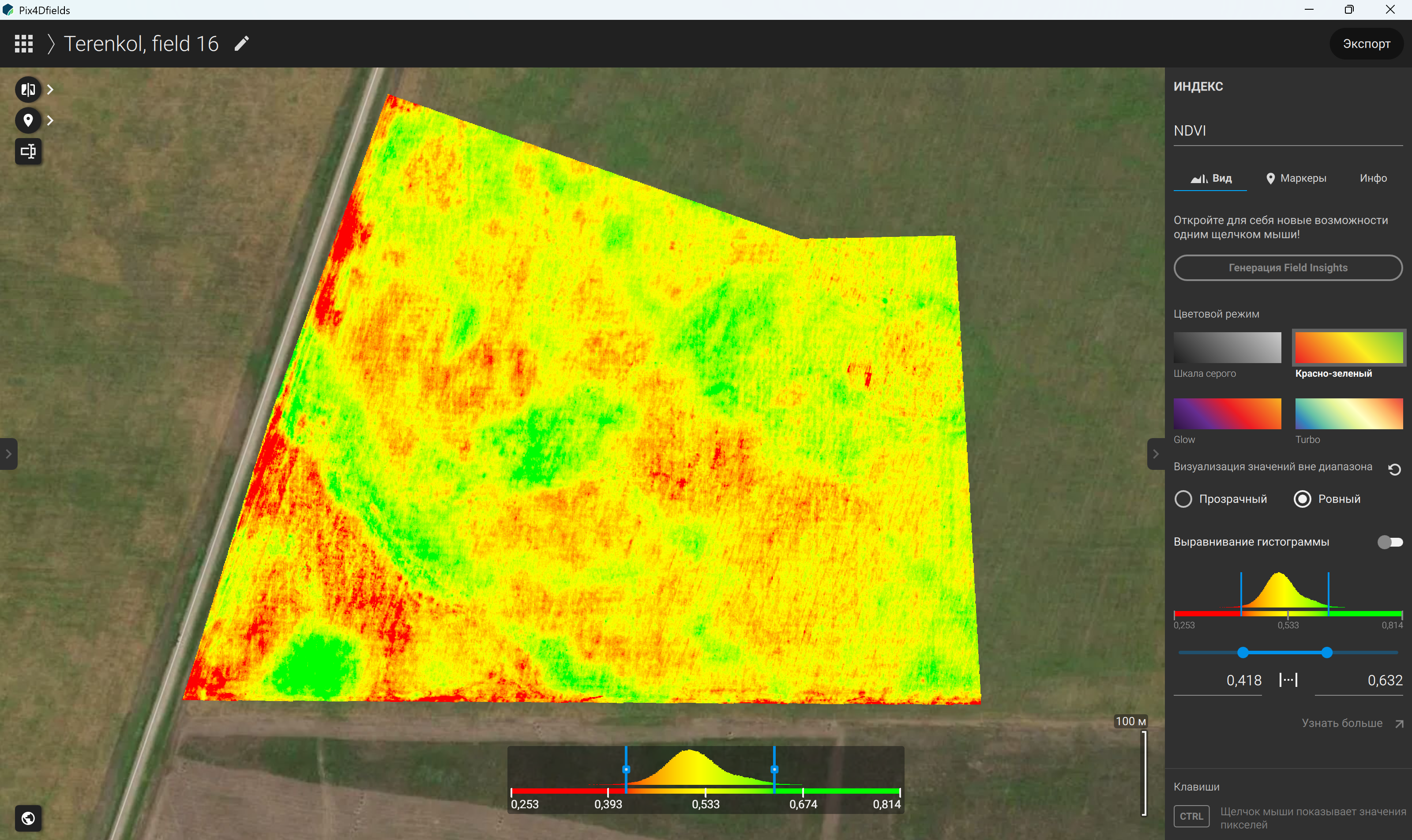
Figure 138 – “Export” command in the top menu bar

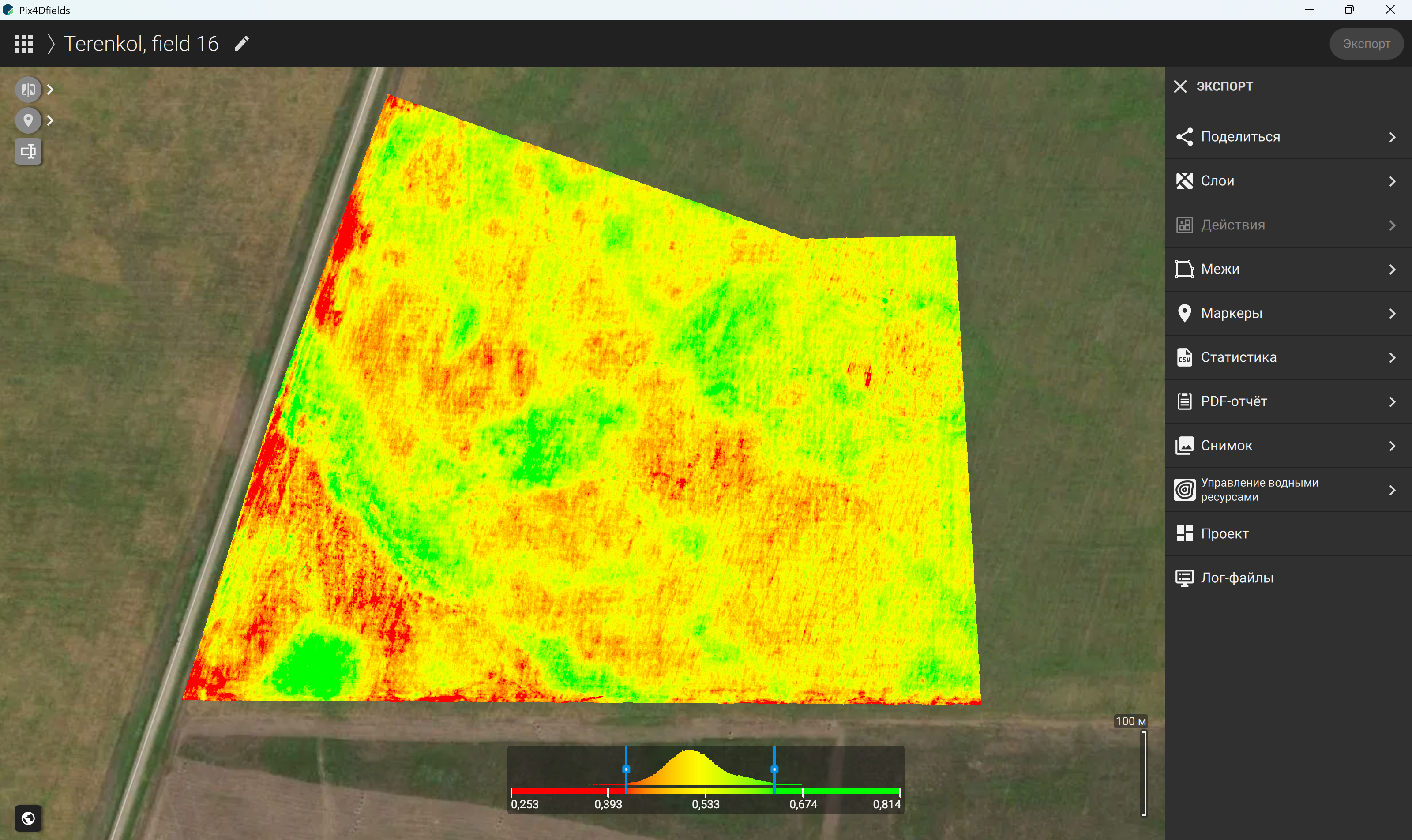
Figure 139 – “Export” settings sidebar

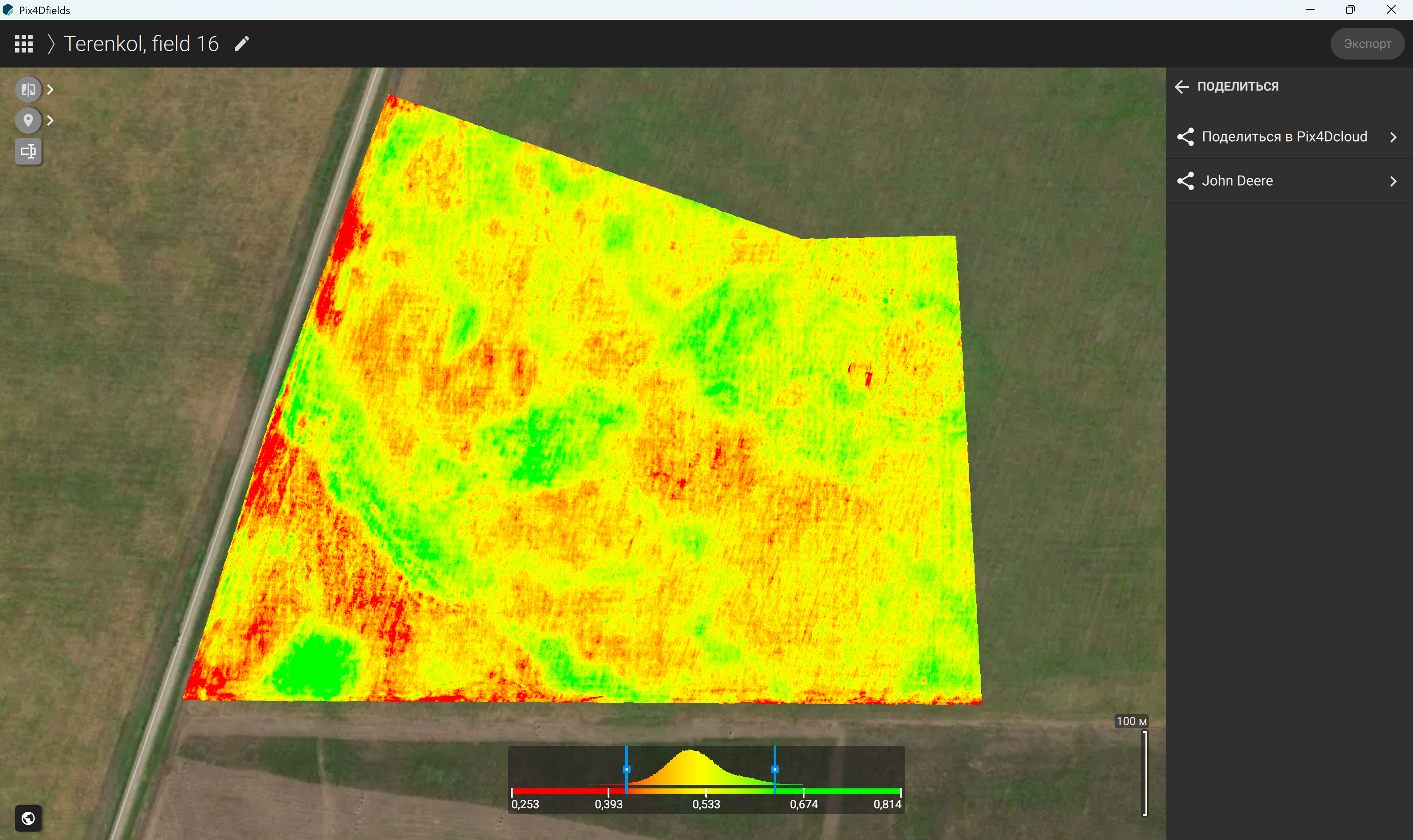
Figure 140 – “Share” panel for exporting or sharing processed data

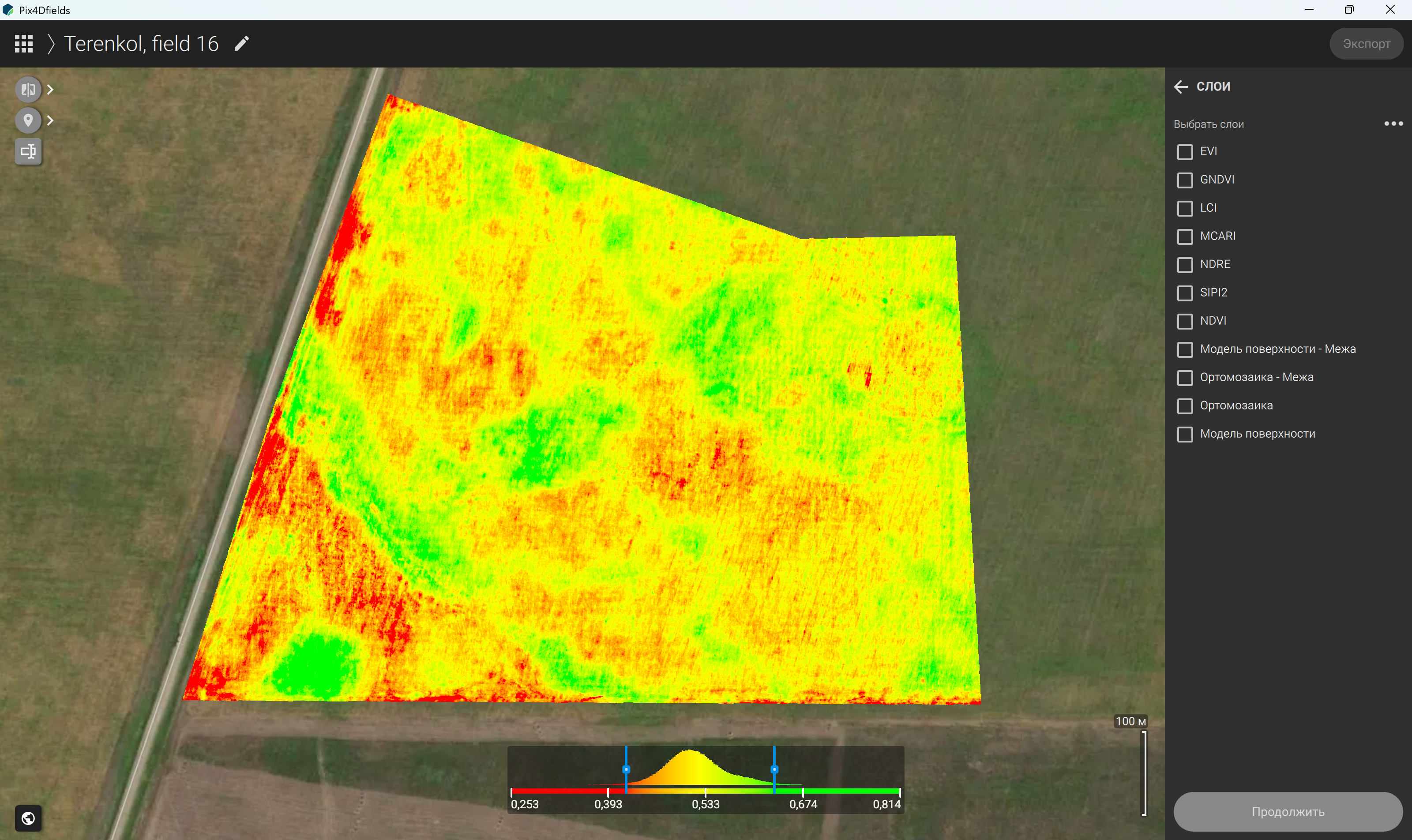
Figure 141 – Selecting layers for export

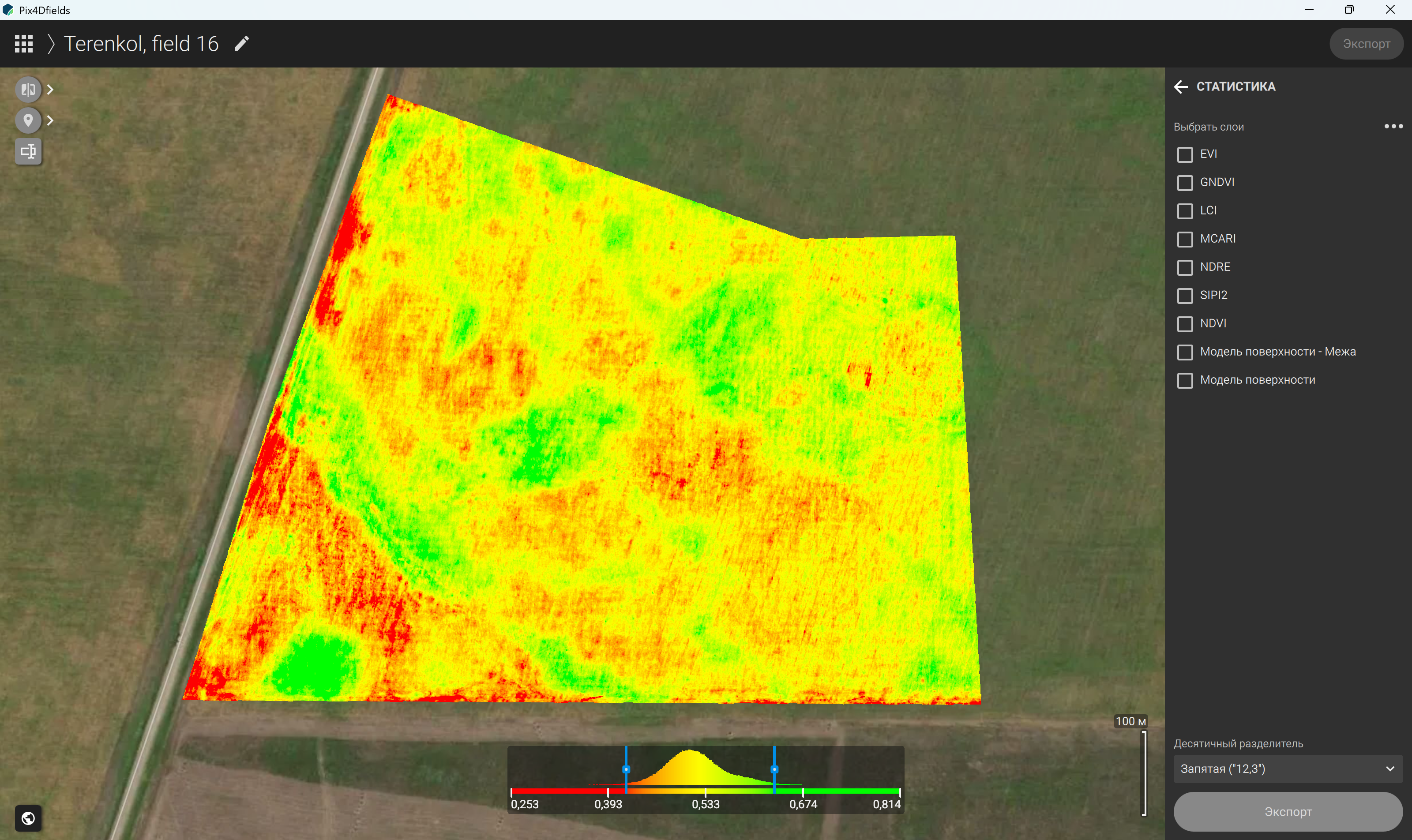
Figure 142 – Exporting layer statistics

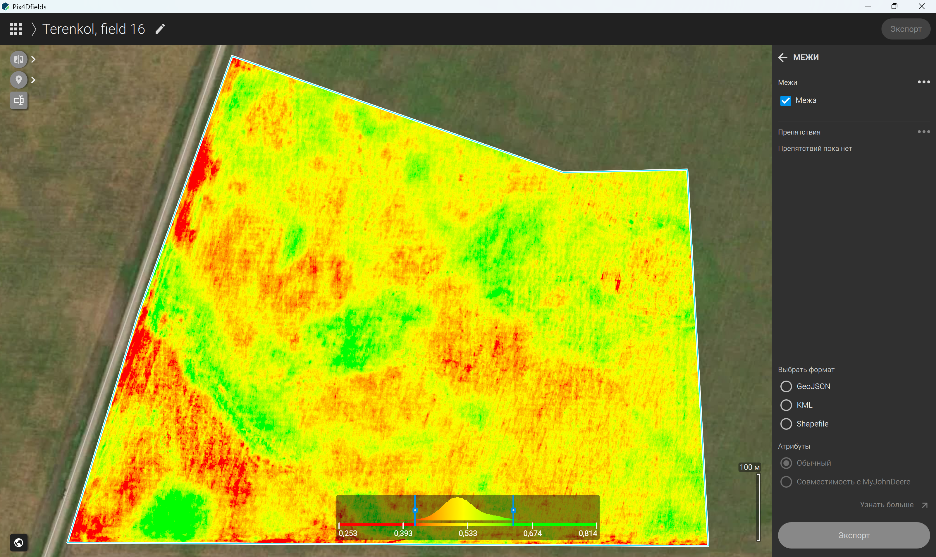
Figure 143 – Selecting field boundaries for export

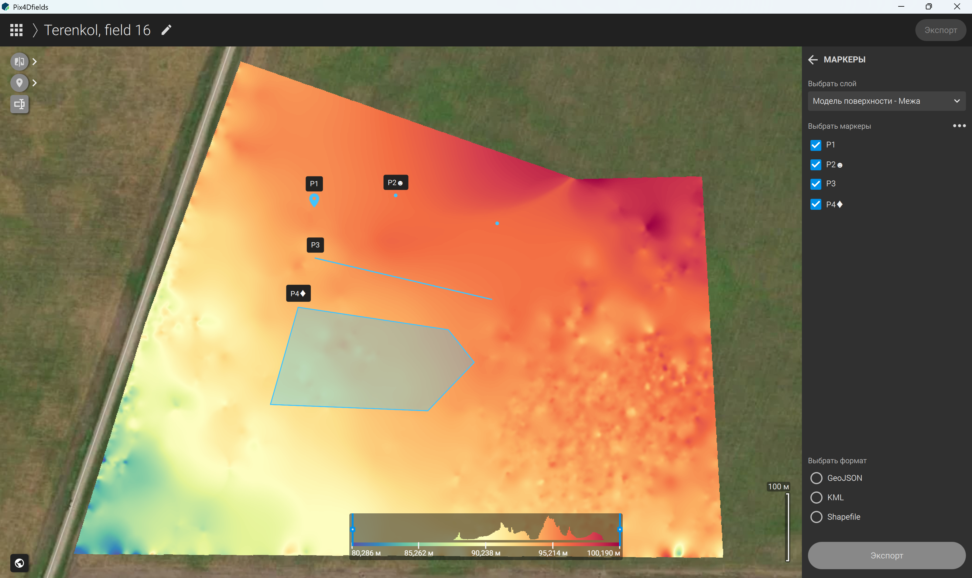
Figure 144 – Selecting annotations and markers for export

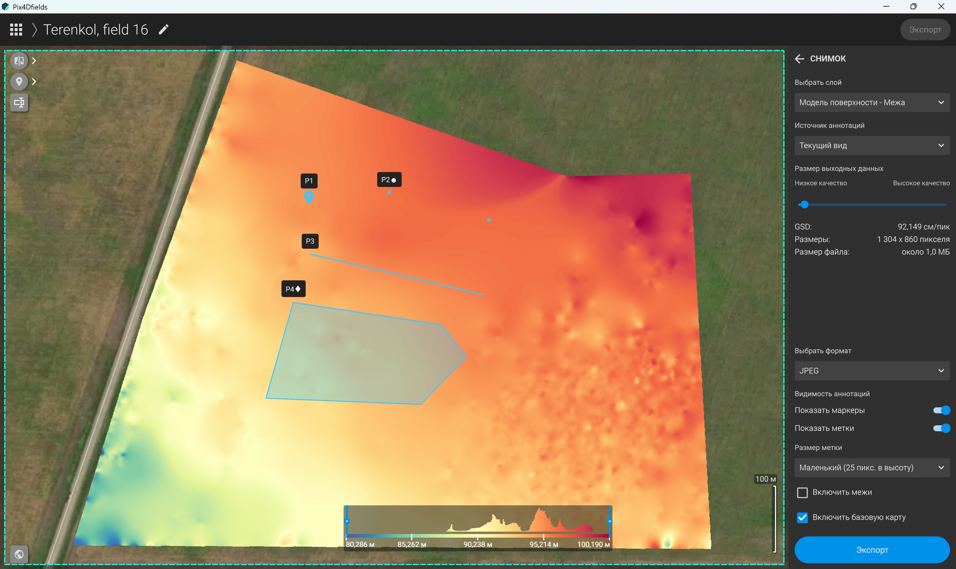
Figure 145 – Configuring image export settings

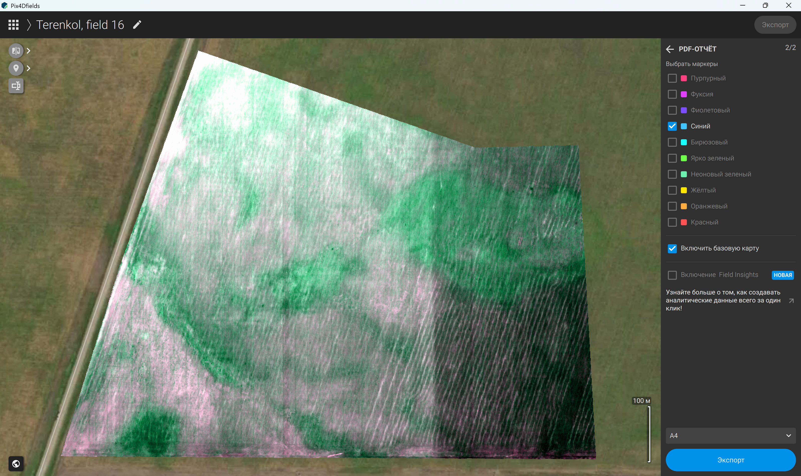
Figure 146 – Selecting markers for export

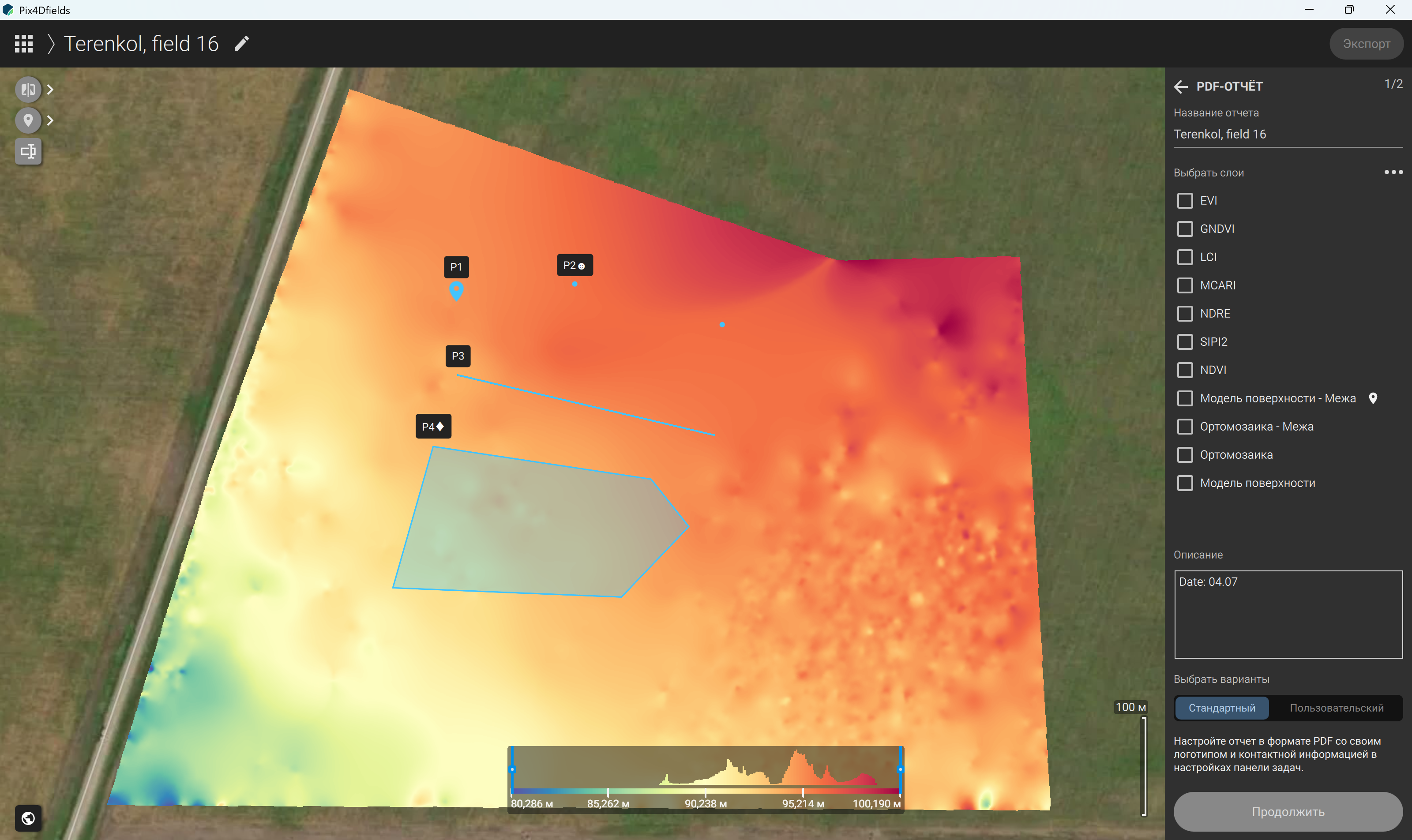
Figure 147 – Selecting the content of a PDF report

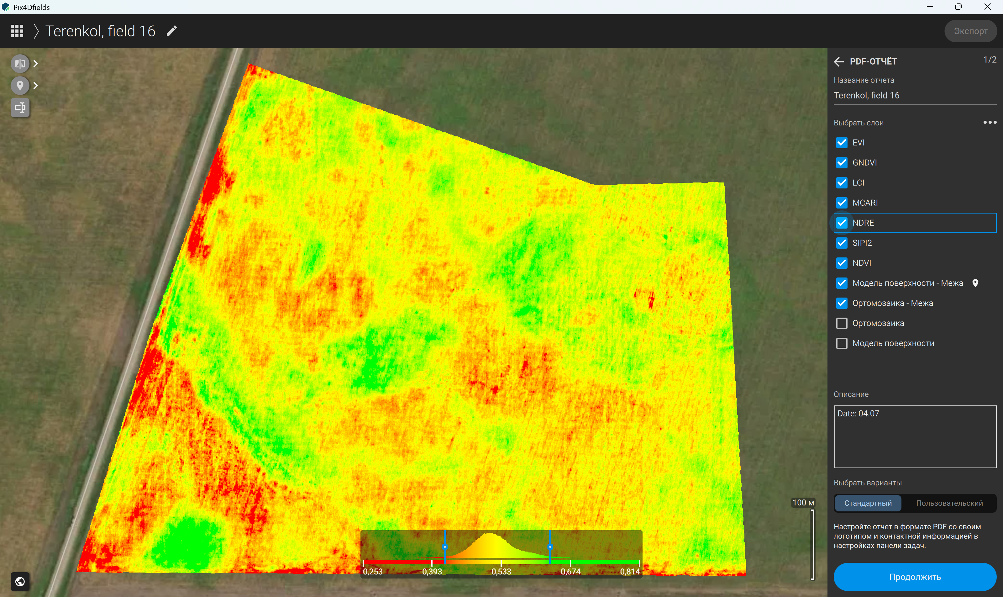
Figure 148 – Selecting report layers and entering the report title and description

The generated report contains detailed information about each selected layer, including maps of the calculated vegetation indices, project details, survey date and time, location, geographic coordinates, and the area of the surveyed territory. For each index, the report may also include a value distribution histogram, a colour legend, visualisation settings, and key statistical indicators.

Following the generation of vegetation index maps, the results are analysed to assess the overall condition of the crops and identify spatial variations in vegetation characteristics. The analysis involves identifying heterogeneous areas within the field and comparing index values across different zones. Based on these findings, areas requiring further investigation can be identified and, where necessary, the field can be divided into management zones according to variations in vegetation conditions. These zones can then be used to develop prescription maps for variable-rate applications of fertilisers and plant protection products. The resulting maps can also be exported in formats compatible with precision agriculture software and machinery, subject to the requirements of the relevant systems.

Thus, the analysis of vegetation indices provides valuable information about crop conditions and vegetation development, helping to identify areas that may exhibit signs of stress, water deficiency, or nutrient imbalances. These findings can inform recommendations for appropriate agronomic measures, including adjustments to fertiliser application rates, irrigation scheduling, and targeted field inspections. By interpreting the observed patterns in the context of crop growth stages and environmental conditions, it becomes possible to distinguish temporary variations in vegetation characteristics from potential problems requiring corrective action. Furthermore, the assessment of vegetation indices can support the evaluation of crop responses to existing management practices and help determine whether additional monitoring or changes in cultivation techniques are warranted. Additional field assessments may be necessary to determine the underlying causes of the detected anomalies and to ensure that subsequent management decisions are appropriate. Such assessments may include visual inspections of plants, examination of soil conditions, and verification of irrigation system performance. Combining remote sensing observations with field-based evidence enables a more comprehensive interpretation of crop conditions and reduces the risk of implementing agronomic measures based solely on spectral information.